the image histogram (v) – tone

May 27, 2022 / spqr / Leave a comment

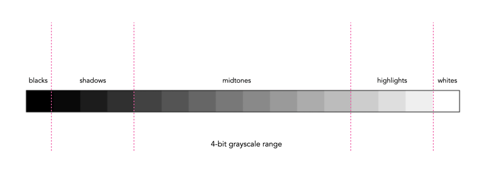
In addition to shape, a histogram can be described using different tonal regions. The left side of the histogram represents the darker tones, or shadows, whereas the right side represents the brighter tones, or highlights, and the middle section represents the midtones. Many different examples of histograms displaying these tonal regions exist. Figure 1 shows a simplified version containing 16 different regions. This is somewhat easier to visualize than a continuous band of 256 grayscale values. The histogram depicts the movement from complete darkness to complete light.

Fig.1: *An example of a tonal range – 4-bit (0-15 gray levels)e*

The tonal regions within a histogram can be described as:

highlights – The areas of a image which contain high luminance values yet still contain discernable detail. A highlight might be specular (a mirror-like reflection on a polished surface), or diffuse (a refection on a dull surface).
mid tones – A midtone is an area of an image that is intermediate between the highlights and the shadows. The areas of the image where the intensity values are neither very dark, nor very light. Mid-tones ensure a good amount of tonal information is contained in an image.
shadows – The opposite of highlights. Areas that are dark but still retain a certain level of detail.

Like the idealized view of the histogram shape, there can also be a perception of an idealized tonal region – the midtones. However an image containing only midtones tends to lack contrast. In addition, some interpretations of histograms add additional an additional tonal category at either extreme. Both can contribute to clipping.

blacks – Regions of an image that have near-zero luminance. Completely black areas are a dark abyss.
whites – Regions of an image where the brightness has been increased to the extent that highlights become “blown out”, i.e. completely white, and therefore lack detail.

Figure 2 shows an image which illustrates nearly all the regions (with a very weird histogram). The numbers on the image indicate where in the histogram those intensities exist. The peak at ① shows the darkest regions of the image, i.e. the deepest shadows. Next, the regions associated with ② include some shadow (ironically they are in shadow), graduating to midtones. The true mid-tonal region, ③, are regions of the buildings in sunlight. The highlights, ④, are almost completely attributed to the sky, and finally there is a “white” region, ⑤, signifying a region of blow-out, i.e. where the sun is reflecting off the white-washed parts of the building.

Fig.2: *An example of the various tonal regions in an image histogram*

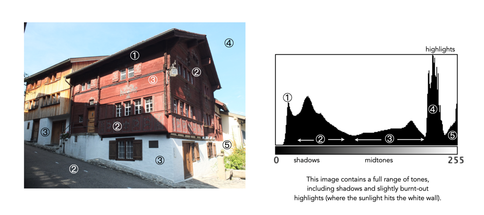
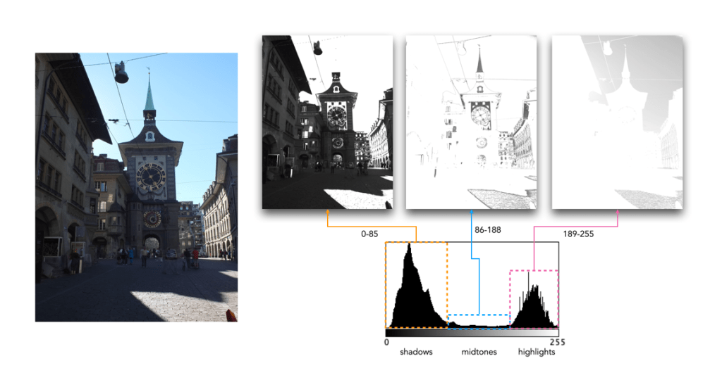
Figure 3 shows how tonal regions in a histogram are associated with pixels in the image. This image has a bimodal histogram, with the majority of pixels in one of two humps. The dominant hump to the left, indicates a good portion of the image is in the shadows. The right-sided smaller hump is associated with the highlights, i.e. the sky, and sunlit pavement. There is very little in the way of midtones, which is not surprising considering the harsh lighting in the scene.

Fig.3: *Tonal regions associated with image regions.*

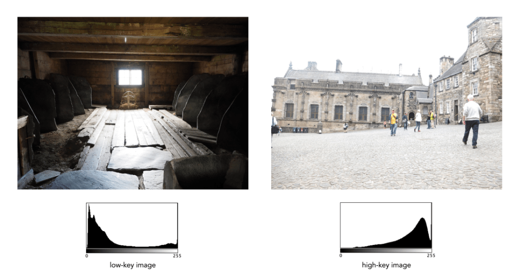
Two other commonly used terms are low-key and high-key.

A high-key image is one composed primarily of light tones, and whose histogram is biased towards 255. Although exposure and lightning can influence the effect, a light-toned subject is almost essential. High-key pictures usually have a pure or nearly pure white background, for example scenes with bright sunlight or a snowy landscape. The high-key effect requires tonal graduations, or shadows, but precludes extremely dark shadows.
A low-key image describes one composed primarily of dark tones, where the bias is towards 0. Subject matter, exposure and lighting contribute to the effect. A dark-toned subject in a dark-toned scene will not necessarily be low-key if the lighting does not produce large areas of shadow. An image taken at night is a good example of a low-key image.

Examples are shown in Figure 4.

Fig.4: *Examples of low-key and high-key images.*

Why did 35mm photography become so popular?

May 18, 2022May 19, 2022 / spqr / Leave a comment

Everything in modern digital photography seems to hark back to analogue 35mm. The concept of “full-frame” only exists because a full frame sensor is equivalent in size to the 24×36mm frame of 35mm film (which was only called 35mm because that was the width of the film). If we didn’t have this association, there would be no crop-sensor. Most early films for cameras were quite large format – introduced in 1899, 116 format film was 70mm wide. This was followed in 1901 by 120 (60mm), 127 (40mm) in 1912, and then 620 (60mm) in 1931. So there were certainly many film format options. So why did 35mm become the standard?

In all likelihood, 35mm became the gold standard because of how widely available 35mm film was in the motion picture industry – it had been around since 1889 when Thomas Edison’s assistant, William Kennedy Dickson simply split 70mm Eastman Kodak film in half. (I have discussed the origins of 35mm film in a previous post). Kodak introduced the standard 135 film in 1934, and was designed for making static pictures (rather than film) with the actual exposure frames being 36mm wide, and 24mm high, giving it a 3:2 ratio. In the 1930s, Leica brochures expounded the fact that the film used in their cameras was “…the standard 35mm cinema film stock, obtainable all over the world.“

*A standard Leica with a 50mm f/3.5 ELMAR lens*

There was much hype in the 1930s about the cameras that were termed “minicams”, or “candid cameras”, in effect cameras that used 35mm film. By the mid 1930s, Leica had been producing 35mm cameras for over a decade. A 1936 Fortune Magazine article titled “The U.S. Minicam Boom” described the Leica as a camera which “took thirty-six pictures the size of the special-delivery stamp on a roll of movie film.” There were those who did not think the miniature camera would survive, seeing their use as a form of candid camera craze. Take for example the closing argument of Thomas Uzzell, who wrote the negative perspective of a 1937 article “Will the Miniature Survive the Candid Camera Craze?” [1]:

“The little German optical jewels you carry in your (sagging) coat pockets make many experimental exposures expensive (though perhaps they would do better if they carefully made one good one!). Their shorter focal lengths make the ultra-fast exposures more practical (how many pictures are actually taken at these ultra speeds!). You can hop about quickly, minnie in hand, and take photos of children and babies at play with all the detail that “makes a picture pulse with naturalness and life” (though good pictures have never been taken by anyone hoping about). … I claim there is just one thing they cannot do, and apparently are never going to be able to do. They can’t make clear pictures.”

Uzzell claimed the art of the miniature was the art of the fuzzy picture. His challenger, Homer Jensen on the other hand described the inherent merits of 35mm over larger format cameras, namely that one could “…take pictures under the most unfavourable conditions, indoors and outdoors.”. Some people disliked the minicam because it made it too easy to take pictures (like anyone could take pictures).

One of the reasons 35mm was so successful was the small size of the camera itself. Their lightweight nature made them easy to carry, taking up very little room. This made them popular with both causal photographers and professionals such as photojournalists where the use of bulky equipment would be prohibitive. Another reason was the 35mm camera’s ability to work in existing light conditions. This was an affect of having ultra-fast lenses, something the larger format cameras could not practically achieve. The shorter focal lengths of 35mm cameras also allowed for greater depth-of-field at wide lens apertures. The inaugural issue of Popular Photography in 1937 described the advantages of using miniatures to capture fast action [4].

*A large format Graflex camera versus a Leica “minicam”.*

Large format cameras on the other hand, were sometimes referred to as “Big Berthas” due to their size [4]. The Series D Graflex, a quintessential 4×5″ press camera of the 1930s weighed 3.06kg, compared with the Leica G, which was one-sixth its weight, and roughly 1/30th its size. In a Graflex brochure from 1936, photographer H. Armstrong Roberts recalls a recent 14,000 mile journey where he took 3000 negatives using his Graflex camera, stating that “Certain I am that no other camera could have achieved the results which I have obtained with the GRAFLEX.”

In 1935, another event foreshadowed the success of 35mm photography – Kodak’s introduction of Kodachrome colour film, followed shortly afterwards by Agfa’s Agfacolor Neu. This may have persuaded many a professional photographer to move to 35mm. Indeed, by 1938, H. Armstrong Roberts was also shooting in colour using a Zeiss Contaflex with a 50mm f/2 Sonnar lens [5] (so much for his belief in large format). The onset of WW2 brought a halt to the first minicam boom, but it was not the end of the story. By the early 1950s, the minicam was on the cusp of greatness, soon to become the standard means of taking photographs. More articles started to appear in photography magazines, enunciating the virtues of 35mm [3].

There are many reasons 35mm film became the format of choice.

Kodak’s 135 film single-use cartridge allowed for daylight loading. Prior to this 35mm film had to be loaded onto reusable cassettes in the darkroom.
The physical format of 35mm film made it very user friendly. The film is contained in a metal canister that reduces the risk of light leaks, and is easy to handle. Loading/unloading film is both intuitive, quick and easy. It’s compact size made it much easier to handle than larger format film.
35mm also allowed for more exposures per roll than typical large format films. The norm is 24 or 36 exposures. This provided a great deal of flexibility in the amount of shots that could be taken, because 35mm film was easier and cheaper to develop.
In the hey-day of film photography there was a huge selection of film types – B&W, colour, infrared, and slide.

Of course there were also some limitations, but these mostly centre on the fact that 35mm film was considered to have less resolving power than medium-format film – great for “snapshots”, but anyone that required large prints needed a large film format to avoid grainy prints.

The invention of the Leica started a new era in photography, spurned on by the introduction of Kodak’s 135 film. Post WW2, 35mm film spearheaded the photographic revolution of the 1950s. It became the format used by amateurs, hobbyists, and professionals alike. 35mm photography allowed for a light, yet flexible kit, which was ideal for the travelling amateur photographer of the 1960s.

The human visual system : focus and acuity

May 16, 2022 / spqr / 1 Comment

There is a third difference between cameras and the human visual system (HVS). While some camera lenses may share a similar perspective of the world with the HVS with respect to the angle-of view, where they differ is what is actually in the area of focus. Using any lens on a camera means that a picture will have an area where the scene is in-focus, with the remainder being out-of-focus. This in-focus region generally occurs in a plane, and is associated with the depth-of-field. On the other hand, the in-focus region of the picture our mind presents us does not have a plane of focus.

While binocular vision allows approximately 120° of (horizontal) vision, it is only highly focused in the very centre, with the remaining picture being increasingly out-of-focus depending on how far a point is away from the central focused region. This may be challenging to visualize, but if you look at an object, only the central point is in focus, the remainder of the picture is out-of-focus. That does not mean it is necessarily blurred, because the brain is still able to discern shape and colour, just not fine details. Blurring it usually a function of distance from the object being focused on, i.e. the point-of-focus. If you look at a close object, distant objects will be out-of-focus, and vice versa.

Focused vision is related to the different parts of the macula, an oval-shaped pigmented area in the centre of the retina which is responsible for interpreting vision, colour, fine details, and symbols (see Figure 1). It is composed almost entirely of cones, into a series of zones:

perifovea (5.5mm∅, 18°) : Details that appear in up to 9-10° of visual angle.
parafovea (3mm∅, 8°) : Details that appear in peripheral vision, not as sharp as the fovea.
fovea (1.5mm∅, 5°) : Or Fovea centralis, comprised entirely of cones, and responsible for high-acuity, and colour vision.
foveola (0.35mm∅, 1°) : A central pit within the fovea, which contains densely packed cones. Within the foveola is a small depression known as the umbo (0.15mm∅), which is the microscopic centre of the foveola.

Fig.2: *Angle-of-view of the whole macula region, versus the foveola.* *The foveola provides the greatest region of acuity*, *i.e. fine details.*

When we fixate on an object, we bring an image of that object onto the fovea. The foveola provides the greatest amount of visual acuity, in the area 1-2° outwards from the point of fixation. As the distance from fixation increases, visual acuity decreases quite rapidly. To illustrate this effect, try reading the preceding text in this paragraph while fixating on the period at the end of the sentence. It is likely challenging, if not impossible, to read text outside a small circle of focus from the point of fixation. A seven letter word, like “outside”, is about 1cm wide, which when read on a screen 60cm from your eye represents about an angle of 1°. The 5° of the fovea region allows for a “preview” of the words either side, and parafovea region, 8° of peripheral words (i.e. their shape). This is illustrated in Figure 3.

To illustrate how this differential focus affects how humans view a scene, consider the image shown in Figure 4. The point of focus is a building in the background roughly 85m from where the person is standing. This image has been modified by adding radial blur from a central point-of-focus to simulate in-focus versus out-of-focus regions as seen by the eye (the blur has been exaggerated). The sharpest region is the point of fixation in the centre – from this focus on a particular object, anything either side of that object will be unsharp, and the further away from that point, the more unsharp is becomes. The

Fig.4: *A simulation of focused versus out-of-focus regions in the HVS (the point of fixation is roughly 85m from the eyes)*

It is hard to effectively illustrate exactly how the HVS perceives a scene as there is no way of taking a snapshot and analyzing it. However we do know that focus is a function of distance from the point-of-focus. Other parts of an image as essentially de-emphasized, there is still information there, and the way our minds process it, it provides a complete vision, but there is a central point of focus.

the image histogram (iv) – shape

May 12, 2022May 27, 2022 / spqr / Leave a comment

One of the most important characteristics of a histogram is its shape. A histogram’s shape offers a good indicator of an image’s ability to tolerate manipulation. A histogram shape can help elucidate the overall contrast in the image. For example a broad histogram usually reflects a scene with significant contrast, whereas a narrow histogram reflects less contrast, with an image which may appear dull or flat. As mentioned previously, some people believe an “ideal” histogram is one having a shape like a hill, mountain, or bell. The reality is that there are as many shapes as there are images. Remember, a histogram represents the pixels in an image, not their position. This means that it is possible to have a number of images that look very different, but have similar histograms.

The shape of a histogram is usually described in terms of simple shape features. These shape features are often described using geographical terms (because a histogram often reminds people of the profile view of a geographical feature): e.g. “hillock” or “mound”, which is a shallow, low feature, “hill” or “hump”, which is a feature rising higher than the surrounding areas, a “peak”, which is a feature with a distinctly top, a “valley”, which is a low area between two peaks, or a “plateau” which is a level region between other features. Features can either be distinct, i.e. recognizably different, or indistinct, i.e. not clearly defined, often blended with other features. These terms are often used when describing the shape of a particular histogram in detail.

Fig.1: *A sample of feature shapes in a histogram*

From the perspective of simplicity, however histogram shapes can be broadly classified into three basic categories (examples are shown in Fig.2):

Unimodal – A histogram where there is one distinct feature, typically a hump or peak, i.e. a good amount of an image’s pixels are associated with the feature. The feature can exist anywhere in the histogram. A good example of a unimodal histogram is the classic “bell-shaped” curve with a prominent ‘mound’ in the center and similar tapering to the left and right (e.g. Fig.2: ①).
Bimodal – A histogram where there are two distinct features. Bimodal features can exist as a number of varied shapes, for example the features could be very close, or at opposite ends of the histogram.
Multipeak – A histogram with many prominent features, sometimes referred to as multimodal. These histograms tend to differ vastly in their appearance. The peaks in a multipeak histogram can themselves be composed of unimodal or bimodal features.

These categories can can be used in combination with some qualifiers (numeric examples refer to Figure 2). For example a symmetric histogram, is a histogram where each half is the same. Conversely an asymmetric histogram is one which is not symmetric, typically skewed to one side. One can therefore have a unimodal, asymmetric histogram, e.g. ⑥ which shows a classic “J” shape. Bimodal histograms can also be asymmetric (⑪) or symmetric (⑬).

Fig.2: *Core categories of histograms: unimodal, bimodal, multi-peak and other.*

Histograms can also be qualified as being indistinct, meaning that it is hard to categorize it as any one shape. In ㉓ there is a peak to the right end of the histogram, however the major of the pixels are distributed in the uniform plateau to the right. Sometimes histogram shapes can also be quite uniform, with no distinct groups of pixels, such as in example ㉒ (in reality though these images are quite rare). It it also possible that the histogram exhibits quite a random pattern, which might only indicate quite a complex scene.

But a histogram’s shape is just its shape. To interpet a histogram requires understanding the shape in context to the contents of the scene within the image. For example, one cannot determine an image is too dark from a left-skewed unimodal histogram without knowledge of what the scene entails. Figure 3 shows some sample colour images and their corresponding histograms, illustrating the variation existing in histograms.

Fig.3: *Various colour images and their corresponding intensity histograms*

The human visual system : image shape and binocular vision

May 3, 2022May 3, 2022 / spqr / Leave a comment

There are a number of fundamental differences between a “normal” 50mm lens and the human visual system (HVS). Firstly, a camera extracts a rectangular image from the circular view of the lens. The HVS on the other hand is not circular, nor rectangular – if anything it has somewhat of an oval shape. This can be seen in the diagram of binocular field of vision shown in Figure 1 (from [1]). The central shaded region is the field of vision seen by both eyes, i.e. binocular (stereoscopic) vision, the white areas on both sides are the monocular crescents, seen by only by each eye, and the blackened area is not seen.

Fig.1: *One of the original diagrams illustrating both the shape of vision, and the extent of binocular vision* [1].

Figure 1 illustrates a second difference, the fact that normal human vision is largely binocular, i.e. uses both eyes to produce an image, whereas most cameras are monocular. Figure 2 illustrates binocular vision more clearly, comparing it to the total visual field.

Fig.2: *Shape and angle-of-view, total versus binocular vision (horizontal).*

The total visual field of the HVS is 190-200° horizontally, which is composed of 120° of binocular vision, and two fields of 35-40° seen by one one eye. Vertically, the visual field of view is about 130° (and the binocular field is roughly the same), comprised of 50° above the horizontal line-of-sight, and 70-80° below it. An example to illustrate binocular vision (horizontal) is shown in Figure 3.

Fig.3: *A binocular (horizontal – 120°) view of Bergen, Norway*

It is actually quite challenging to provide an exact example of what a human sees – largely because trying to take the same picture would require a lens such as a fish-eye which would introduce distortions, something the HVS is capable of filtering out.

The glass beans – the origin of “lens”

April 28, 2022 / spqr / Leave a comment

When lenses first appeared they had a particular shape, a double convex lens, that was very similar to a certain pulse, namely the lentil. The name lens derived from the Latin name for the plant, lens culinaris.

“LENS (Latin , lens, a small bean or lentil). A lens is a piece of transparent material (usually glass) bounded by curved surfaces (generally spherical, including flat).
A.L.M. Sowerby’s Dictionary of Photography (1951) p.407

An English dictionary of the early 18th century [1] describes a lens as related to optics to be a “small concave or convex glass”. By 1768 [2] it was described as “a glass, spherically convex on both sides”.

The word lentil comes from the Old French lentille, which in turn comes from Latin lenticula. When lenses first appeared, they looked like the lentil seed, and likely due to the fact that technical terms were derived from Greek or Latin, simply named them lens. In German, one term used is Linse, but it is more common to use the term Objektiv. The term Linse is from the Old High German linsa, from a Proto-Indo-European root.

Dictionarium Anglo-Britannicum, John Kersey (1708)
A Dictionary of the English Language, Samuel Johnson (1768)

Why was the 50mm lens considered “normal”?

April 22, 2022September 6, 2022 / spqr / 3 Comments

Why was the 50mm lens considered the “normal” lens used on 35mm cameras? Why not 40mm or 60mm? When Barnack introduced his revolutionary Leica camera, he used a traditional method of selecting the lens – the most commonly used lens has a focal length should be approximately equal to the diagonal of the negative, which is how the 50mm likely evolved. The Leica I came with a fixed 50mm lens, and even when the Leica II appeared in 1932 with interchangeable lenses, the viewfinder was designed to work with 50mm lenses. Zeiss Contax lens brochures from the 1930s mark 50mm lenses as “universal lenses”, “For all-round use and subjects which occur in every-day photography…”. Nikon also made the point that “Nikkor normal lenses cover a picture angle of approximately 45°, corresponding closely to the angle of view of the human eye”.

It is then no surprise that 50mm is the most ubiquitous analog lens. By the 1950s, most interchangeable lens cameras came standard with a 50mm lens, ensuring that novice photographers could capture sharp photographs in a variety of conditions without requiring a books worth of knowledge. Nikon in one of their lens brochures suggested “the 50mm focal length has become the standard lens for all around work”. This deep-seeded ideology is probably why 50mm lenses came in so many speeds – the same Nikon brochure provides an f/3.5, f/2, f/1.4, and f/1.1 50mm lenses. Many camera manufacturers followed suit. The late 1970s “standard” line-up for Asahi Pentax included four 50mm lenses (f/1.2, f/1.4, f/1.7, f/2) and a 40mm f/2.8 which they touted as being “extremely versatile”.

Fig.1: *How many normal’s is too many normal’s? (Pentax SMC lenses)*

There are a number of arguments that have traditionally been made as to why 50mm is “normal”. The most common argument of course is that the 50mm lens has a diagonal angle-of-view (AOV) of about 45° which approximates the AOV of the human eye. But in reality it makes assumptions about what “normal vision” is , and the ability of a 50mm lens to reproduce it. The idea that 50mm best approximates human vision has more to do with the evolution of lenses than it has to do with any correspondence between the human eye and a lens. There are other arguments, for instance that 50mm reproduces facial proportions, depth and perspective roughly as how our eyes perceive them. Many manufacturers drove this point home by saying 50mm lenses “give pictures of natural, i.e. normal, perspective”.

Fig.2: *Angle of views of the human vision system*

Firstly we should remember that “normal” human vision is binocular, while camera lenses are not. The eye is also composed of a gel-like material, versus the glass of lens elements. So there are already fundamental structural and functional differences. There is also the matter of AOV. A lens generally has one AOV, whereas the human visual system (HVS) has a series, based on differing abilities to focus – binocular vision is approximately 120° of view, of which only 60° is the central field of vision (the remainder is peripheral vision), and only 30° of that is vision capable of symbol recognition (even less is capable of sharp focusing, perhaps 5°?). Note that I use horizontal AOV in comparisons, because it is easier for people to conceptualize than diagonal AOV.

Fig.3: *AOV of various lens focal lengths against the AOV of the human vision system*

In reference to Figure 3, for the hard limits, a 67mm lens would likely best approximate the 30° region of the HVS that deals with symbol recognition, whereas a 31mm would best approximate the 60° central field of vision. If we were simply to take the middle ground, at 45°, we get a 43mm lens, which actually matches the diagonal of the 24×36mm frame.

But how closely does the 50mm AOV resembles that of the human visual system (HVS)? In terms of horizontal vision, a 50mm lens has a 40° AOV, so it’s not that far removed from that of the 43mm lens. Part of the problem lies with the fact that it is hard to establish an exact value that represents the “normal viewing angle” of the HVS. This is why other lens fit into this “normal” category – the 40mm (48°), the 45mm (44°), the 55mm (36°) and the 58mm (34°). Herbert Keppler may have put it best in his book The Asahi Pentax Way (1966):

“A normal focal length lens on any camera is considered to be a lens whose focal length closely approximates the diagonal of the picture area produced on the film. With 35mm cameras, this actually works out to be about 43mm, generally considered a little too short to produce the best angle of coverage and most pleasing perspective. Consequently, makers of 35mm cameras have varied their “normal” focal lengths between 50 and 58mm. With early single lens reflexes the longer 58mm length was in general use. However, in recent years there seems to be a trend to slightly shorter focal lengths which produce a greater angle of view. Current Pentax models use both 50 and 55mm focal length lenses.”

In some respects it seems like 50mm was chosen because it is close to what could be perceived as the AOV of the HVS, such that it is, and provided a nice rounded focal length value. By the 1950s, the 50mm had become “the standard” lens, with 35mm and 85mm lenses providing wide and telephoto capabilities respectively (a 35mm lens has an AOV of 54°, and the 85mm lens has an AOV of 24°, and surprisingly, 50mm sits smack dab in the middle of these). Many brochures simply identified it as an “all-round” lens. It is difficult to pinpoint where the reference of 50mm approximating the AOV of the human eye may have first appeared.

With the move to digital, the exact notion of a 50mm “normal” lens has not exactly persevered. This is primarily because the industry has moved away from 36×24mm being the normal film/sensor size, even though we hang onto the idea of 35mm equivalency. While a 50mm lens might be considered “normal” on a full-frame sensor, on an APS-C sensor a “normal” lens would be 35mm, because it is “equivalent” to a 50mm full-frame lens, from the perspective of focal length and more importantly AOV. Note that Zeiss still allude to the fact that the “focal length of the ZEISS Planar T* 1.4/50 is equal to the perspective of the human eye.”

The world is 3D

April 19, 2022November 18, 2022 / spqr / Leave a comment

“The world is three-dimensional; a photographic image is two-dimensional. Because of this flatness, the depth of depictive space always always bears a relationship to the picture plane. The picture plane is a field upon which the lens’s image is projected. A photographic image can rest on this picture plane and, at the same time, contain an illusion of deep space.”
Stephen Shore, The Nature of Photographs

Time and photographs

April 14, 2022April 14, 2022 / spqr / Leave a comment

“There is no such thing as an instantaneous photograph. All photographs are time exposures, of shorter or longer duration, and each describes a discrete parcel of time. This time is always the present. Uniquely in the history of pictures, a photograph describes only that period of time in which it was made. Photography alludes to the past and the future only in so far as they exist in the present, the past through its surviving relics, the future through prophecy visible in the present.”

John Szarkowski, The Photographer’s Eye (1966)

A list of vintage super-fast 50-60mm f/1.2 lenses

April 8, 2022 / spqr / 2 Comments

So who made f/1.2 lenses? The answer is that most manufacturers had some lenses with this large aperture, usually in the 50-60mm range. Most of these lenses came from Japanese manufacturers, who led the way in fast lenses. The only real exception is the Leitz Wetzlar Noctilux 50mm, and they are expensive, to the point where it is cheaper to buy a new Noctilux-M 50mm f/1.2 ASPH (for US$8k).

These lenses are sorted by focal length and years up to 1985. Up until 1975, there were few if any 50mm f/1.2 lenses for SLR cameras, but there were a range of 55/58mm f/1.2 lenses. Note R indicates a lens for a rangefinder camera.

50mm

1954 – Fuji Fujinon 5cm f/1.2 R
1956 – Canon 50mm f/1.2 R
1966 – Leitz Wetzlar Noctilux 50mm f/1.2 R
1975 – Pentax SMC 50mm f/1.2
1978 – Minolta MD Rokkor 50mm f/1.2
1978 – Nikon AI Nikkor 50mm f/1.2
1980 – Canon FDn 50mm f/1.2
1981 – Minolta MD 50mm f/1.2
1981 – Nikon AI-S Nikkor 50mm f/1.2
1981 – Fuji Photofilm EBC X-Fujinon 50mm f/1.2 DM (+Porst UMC)
1982 – Olympus OM Zuiko Auto-S 50mm f/1.2
1984 – SMC Pentax-A 50mm f/1.2

55mm

1962 – Canon R Super-Canomatic 58mm f/1.2
1965 – Nikkor-S Auto f/1.2 55mm
1968 – Canon FL 55mm f/1.2
1970 – Tomioka Auto (Chinon/Cosinon/Revuenon/Yashinon/Cosina) 55mm f/1.2
1970 – Tomioka Kogaku Auto Tominon 55mm f/1.2
1971 – Canon FD 55mm f/1.2 (+AL)
1972 – Olympus OM G.Zuiko Auto-S 55mm f/1.2
1973 – Tomioka Auto Yashinon DS-M 55mm f/1.2
1974 – Nikon Nikkor 55mm f/1.2
1975 – Canon FD 55mm f/1.2 Aspherical
1976 – Yashica ML 55mm f/1.2
1977 – Nikon AI Nikkor 55mm f/1.2

57-60mm

1956 – Konishiroku Hexanon 60mm f/1.2 R
1960 – Tamron 58mm f/1.2
1962 – Canon Super-Canomatic R 58mm f/1.2
1964 – Canon FL 58mm f/1.2
1967 – Konica Hexanon/Hexar 57mm f/1.2
1968 – Minolta MC Rokkor-PG 58mm f/1.2
1973 – Minolta MC Rokkor(-X) PG 58mm f/1.2
1977 – Nicon Noct-Nikkor 58mm f/1.2
1981 – Nikon AI-S Noct_Nikkor 58mm f/1.2

Crafting Pixels

Vintage lenses, photography and digital imagery

the image histogram (v) – tone

Why did 35mm photography become so popular?

Further reading:

The human visual system : focus and acuity

Further reading:

the image histogram (iv) – shape

The human visual system : image shape and binocular vision

Further reading:

The glass beans – the origin of “lens”

Why was the 50mm lens considered “normal”?

The world is 3D

Time and photographs

A list of vintage super-fast 50-60mm f/1.2 lenses

50mm

55mm

57-60mm