Image sharpening – image content and filter types

Using a sharpening filter is really contingent upon the content of an image. Increasing the size of a filter may have some impact, but it may also have no perceptible impact – what-so-ever. Consider the following photograph of the front of a homewares store taken in Oslo.

A storefront in Oslo with a cool font

The image (which is 1500×2000 pixels – down sampled from a 12MP image) contains a lot of fine details, from the stores signage, to small objects in the window, text throughout the image, and even the lines on the pavement. So sharpening would have an impact on the visual acuity of this image. Here is the image sharpened using the “Unsharp Mask” filter in ImageJ (radius=10, mask-weight=0.3). You can see the image has been sharpened, as much by the increase in contrast than anything else.

Image sharpened with Unsharp masking radius=10, mask-weight=0.3

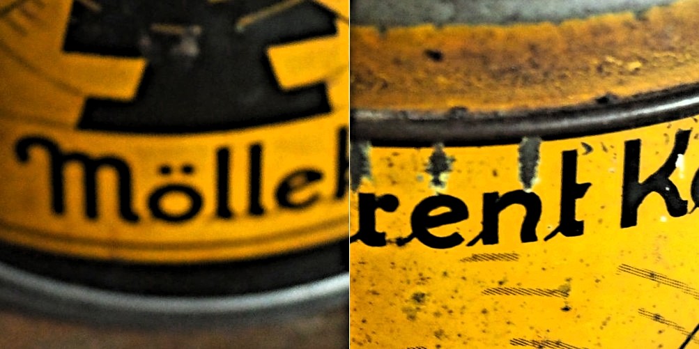
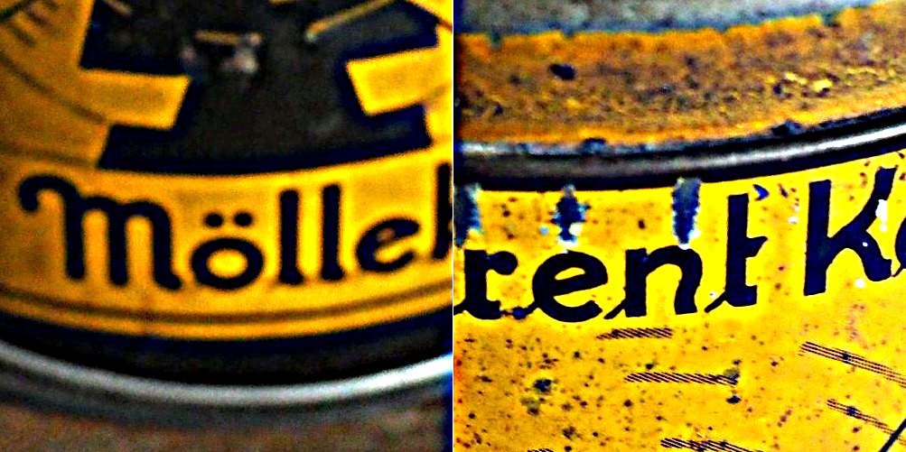
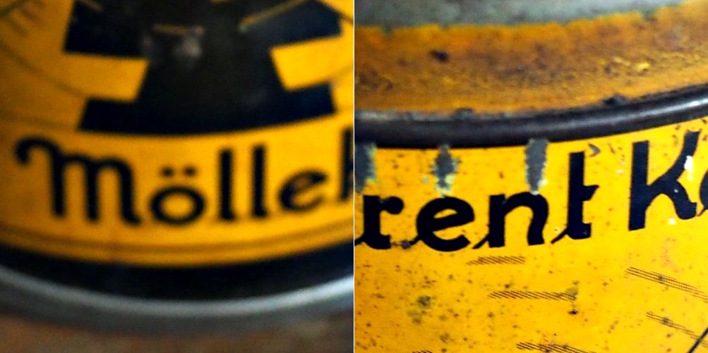
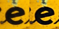
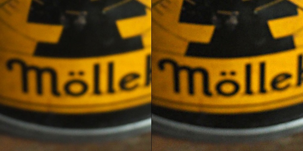
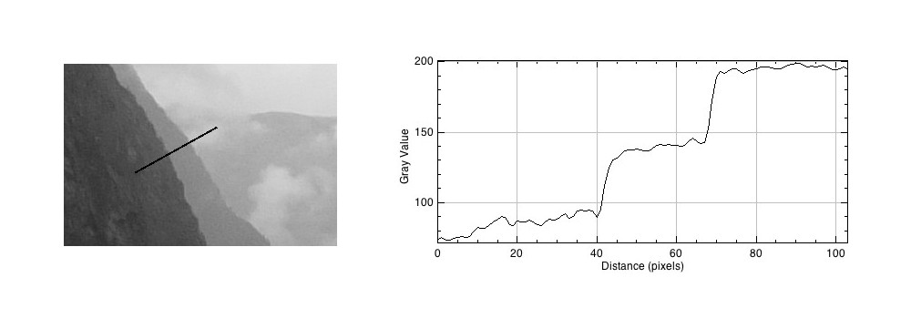
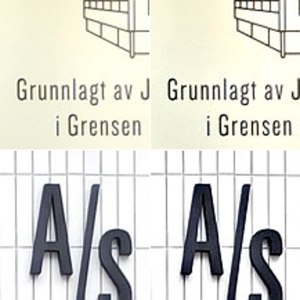
Here is a close-up of two regions, showing how increasing the sharpness has effectively increased the contrast.

Pre-filtering (left) vs. post-sharpening (right)

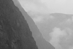
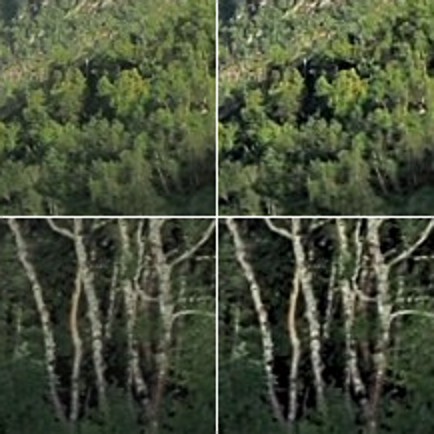
Now consider an image of a landscape (also from a trip to Norway). Landscape photographs tend to lack the same type of detail found in urban photographs, so sharpening will have a different effect on these types of image. The impact of sharpening will be reduced in most of the image, and will really only manifest itself in the very thin linear structures, such as the trees.

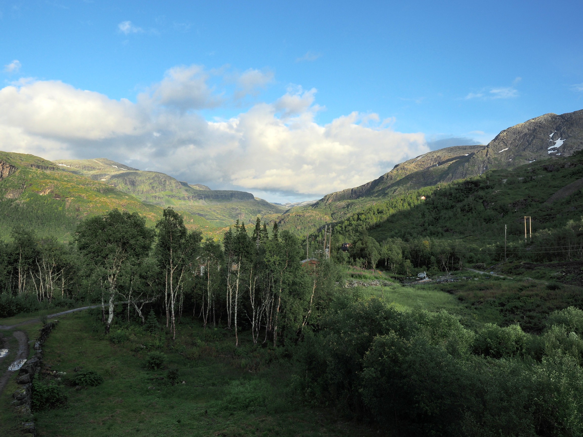
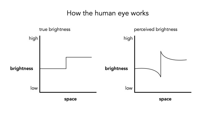
Sharpening tends to work best on features of interest with existing contrast between the feature and its surrounding area. Features that are too thin can sometimes become distorted. Indeed sometimes large photographs do not need any sharpening, because the human eye has the ability to interpret the details in the photograph, and increasing sharpness may just distort that. Again this is one of the reasons image processing relies heavily on aesthetic appeal. Here is the image sharpened using the same parameters as the previous example:

Image sharpened with Unsharp masking radius=10, mask-weight=0.3

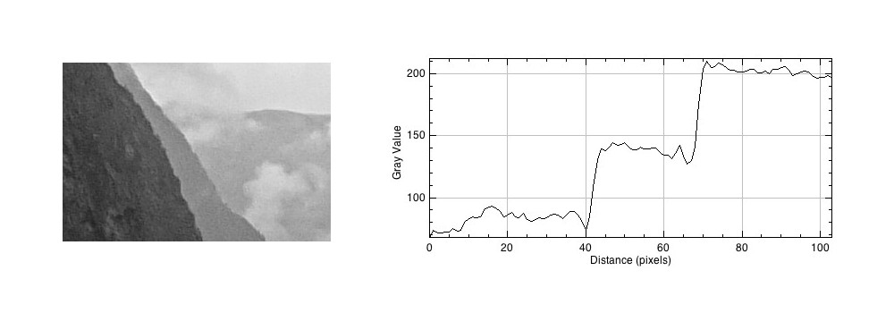
There is a small change in contrast, most noticeable in the linear structures, such as the birch trees.  Again the filter uses contrast to improve acuity (Note that if the filter were small, say with a radius of 3 pixels, the result would be minimal). Here is a close-up of two regions.

Pre-filtering (left) vs. post-sharpening (right)

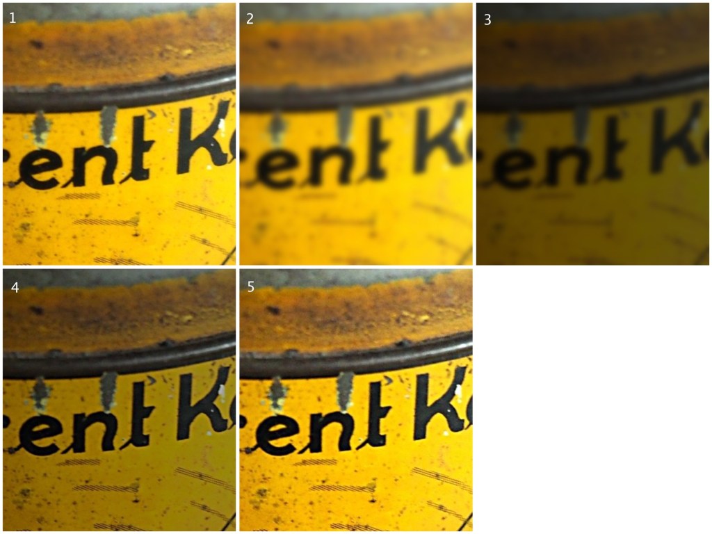
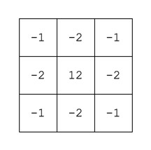
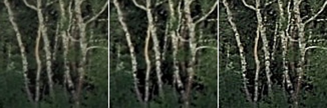
Note that the type of filter also impacts the quality of the sharpening. Compare the above results with those of the ImageJ “Sharpen” filter, which uses a kernel of the form:

ImageJ “Sharpen” filter

Notice that the “Sharpen” filter produces more detail, but at the expense of possibly overshooting some regions in the image, and making the image appear grainy. There is such as thing as too much sharpening.

Original vs. ImageJ “Unsharp Masking” filter vs. ImageJ “Sharpen” filter

So in conclusion, the aesthetic appeal of an image which has been sharpened is a combination of the type of filter used, the strength/size of the filter, and the content of the image.

Image sharpening in colour – how to avoid colour shifts

It is unavoidable – processing colour images using some types of algorithms may cause subtle changes in the colour of an image which affect its aesthetic value. We have seen this in certain forms of the unsharp masking parameters used in ImageJ. How do we avoid this? One way is to create a more complicated algorithm, but the reality is that without knowing exactly how a pixel contributes to an object that’s basically impossible. Another way, which is way more convenient is to use a separable colour space. RGB is not separable – the red, green and blue components must work together to form an image. Modify one of these components, and it will have an affect on the rest of them. However if we use a colour space such as HSV (Hue-Saturation-Value), HSB (Hue-Saturation-Brightness) or CIELab, we can avoid colour shifts altogether. This is because these colour spaces separate luminance from colour information, therefore image sharpening can be performed on the luminance layer only – something known as luminance sharpening.

Luminance,  brightness, or intensity can be thought of as the “structural” information in the image. For example first we convert an image from RGB to HSB, then process only the brightness layer of the HSB image. Then convert back to RGB. For example, below are two original regions extracted from an image, both containing differing levels of blur.

Original “blurry” image

Here is the RGB processed image (UM, radius=10, mask weight=0.5):

Sharpened using RGB colour space

Note the subtle changes in colour in the region surrounding the letters? Almost a halo-type effect. This sort of colour shift should be avoided. Now below is the HSB processed image using the same parameters applied to only the brightness layer:

Sharpened using the Brightness layer of HSB colour space

Notice that there are acuity improvements in both images, however it is more apparent in the right half, “rent K”. The black objects in the left half, have had their contrast improved, i.e. the black got blacker against the yellow background, and hence their acuity has been marginally enhanced. Neither suffers from colour shifts.

Unsharp masking in ImageJ – changing parameters

In a previous post we looked at whether image blur could be fixed, and concluded that some of it could be slightly reduced, but heavy blur likely could not. Here is the image we used, showing blur at two ends of the spectrum.

Blur at two ends of the spectrum: heavy (left) and light (right).

Now the “Unsharp Masking” filter in ImageJ, is not terribly different from that found in other applications. It allows the user to specify a “radius” for the Gaussian blur filter, and a mask weight (0.1-0.9). How does modifying the parameters affect the filtered image? Here are some examples using a radius of 10 pixels, and a variable mask weight.

Radius = 10; Mask weight = 0.25
Radius = 10; Mask weight = 0.5
Radius = 10; Mask weight = 0.75

We can see that as the mask weight increases, the contrast change begins to affect the colour in the image. Our eyes may perceive the “rent K” text to be sharper in the third image with MW=0.75, but the colour has been impacted in such as way that the image aesthetics have been compromised. There is little change to the acuity of the “Mölle” text (apart from the colour contrast). A change in contrast can certainly improve the visibility of detail in the image (i.e. they are easier to discern), however maybe not their actual acuity. It is sometimes a trick of the eye.

What about if we changed the radius? Does a larger radius make a difference? Here is what happens when we use a radius of 40 pixels, and a MW=0.25.

Radius = 40; Mask weight = 0.25

Again, the contrast is slightly increased, and perceptual acuity may be marginally improved, but again this is likely due to the contrast element of the filter.

Note that using a small filter size, e.g. 3-5 pixels in a large image (12-16MP) will have little effect, unless there are features in the image that size. For example, in an image containing features 1-2 pixels in width (e.g. a macro image), this might be appropriate, however will likely do very little in a landscape image.

What is unsharp masking?

Many image post-processing applications use unsharp masking (UM) as their choice of sharpening algorithm. It is one of the most ubiquitous methods of image sharpening. Unsharp masking was introduced by Schreiber [1] in 1970 for the purpose of improving the quality of wirephoto pictures for newspapers. It is based on the principle of photographic masking whereby a low-contrast positive transparency is made of the original negative. The mask is then “sandwiched” with the negative, and the amalgam used to produce the final print. The effect is an increase in sharpness.

The process of unsharp masking accentuates the high-frequency components of an image, i.e. the edge regions where there is a sharp transition in image intensity. It does this by extracting the high-frequency details from an image, and adding them to the original image. This process can be better understood by first considering a 1D signal shown in the figure below.

An example of unsharp masking using a 1D signal

This is the process of what happens to the signal

  1. The original signal.
  2. The signal is “blurred”, by a filter which enhances the “low-frequency” components of the signal.
  3. The blurred signal, ➁, is subtracted from ➀, to extract the “high-frequency” components of the signal, i.e. the “edge” signal.
  4. The “edge” signal is added to the original signal ➀ to produce the sharpened signal.

In the context of digital images unsharp masking works by subtracting a blurred form of an image from the original image itself to create an “edge” image which is then used to improve the acuity of the original image. There are many different approaches to unsharp masking which use differing forms of filters. Some use a more traditional approach using the process outlines above, with the blurring actuated using a Gaussian blur, while others use specific filters which create “edge” images directly, which can be either added to, or subtracted from the original image.

[1] Schreiber, W., “Wirephoto quality improvement by unsharp masking,” Pattern Recognition, Vol.2, pp.117-121 (1970). 

Image enhancement (2) : the fine details (i.e. sharpening)

More important than most things in photography is acuity – which is really just a fancy word for sharpness, or even image crispness. Photographs can be blurry for a number of reasons, but usually they are all trumped by lack of proper focusing, which adds a softness to an image. Now in a 3000×4000 pixel image, this blurriness may not be that apparent – and will only manifest itself when an enlargement is made of a section of the image. In terms of photographing landscapes, the overall details in the image may be crisp, however small objects may “seem” blurry, because they are small, and lack detail in any case. Sharpening will also fail to fix large blur artifacts – i.e. it’s not going to remove defocus from a photograph which was not properly focused. It is ideal for making fine details crisper.

Photo apps and “image editing” software often contains some means of improving the sharpness of images. Usually by means of the “cheapest” algorithm in existence – “unsharp masking”. It works by subtracting  a “softened” copy of an image from the original. And by softened, I mean blurred. It basically reduces the lower frequency components of the image. But it is no magical panacea. If there is noise in an image, it too will be attenuated. The benefit of sharpening can often be seen best on images containing fine details. Here are examples of three different types of sharpening algorithms on an image with a lot of fine detail.

Sharpening: original (top-L); USM (top-R); CUSM (bot-L); MS (bot-R)

Three filters are shown here are (i) Unsharp masking (USM), (ii) Cubic Unsharp masking (CUSM) and (iii) Morphological sharpening (MS). Each of these techniques has its benefits and drawbacks, and the final image with improved acuity can only really be judged through visual assessment. Some algorithms may be more attune to sharpening large nonuniform regions (MS), whilst others (USM, CUSM) may be more aligned with sharpening fine details.

Can blurry images be fixed?

Some photographs contain blur which is very challenging to remove. Large scale blur, which is the result of motion, or defocus can’t really be suppressed in any meaningful manner. What can usually be achieved by means of image sharpening algorithms is that finer structures in an image can be made to look more crisp. Take for example the coffee can image shown below, in which the upper lettering on the label in almost in focus, while the lower lettering has the softer appearance associated with de-focus.

The problem with this image is partially the fact that the blur is not uniform. Below are two regions enlarged:containing text from opposite ends of the blur spectrum.

Reducing blur, involves a concept known as image sharpening(which is different from removing motion blur, a much more challenging task). The easiest technique for image sharpening, and the one most often found in software such as Photoshop is known as unsharp masking. It is derived from analog photography, and basically works by subtracting a blurry version of the original image from the original image. It is by no means perfect, and is problematic in images where there is noise, as it tends to accentuate the noise, but it is simple.

Here I am using the “Unsharp Mask” filter from ImageJ. It subtracts a blurred copy of the image and rescales the image to obtain the same contrast of low frequency structures as in the input image. It works in the following manner:

  1. Obtain a Gaussian blurred image, by specifying a blur radius (in the example below the radius = 5).
  2. Filter the blurred image using a “Mask Weight, which determines the strength of filtering. A value from 0.1-0.9. (In the example below, the mask weight =0.4)
  3. Subtract the filtering image from the original image.
  4. Divide the resulting image by (1.0-mask weight) – 0.6 in the case of the example.
1. Original image; 2. Gaussian blurred image (radius=5); 3. Filtered image (multiplied by 0.4); 4. Subtracted image (original-filtered); 5. Final image (subtracted image / 0.6)

If we compare the resulting images, using an enlarged region, we find the unsharp masking filter has slightly improved the sharpness of the text in the image, but this may also be attributed to the slight enhancement in contrast. This part of the original image has less blur though, so let’s apply the filter to the second image.

The original image (left) vs. the filtered image (right)

Below is the result on the second portion of the image. There is next to no improvement in the sharpness of the image. So while it may be possible to slightly improve sharpness, where the picture is not badly blurred, excessive blur is impossible to “remove”. Improvements in acuity may be more to the slight contrast adjustments and how they are perceived by the eye.

Mach bands and the perception of images

Photographs, and the results obtained through image processing are at the mercy of the human visual system. A machine cannot interpret how visually appealing an image is, because aesthetic perception is different for everyone. Image sharpening takes advantage of one of the tricks of our visual system. Human eyes see what are termed “Mach bands” at the edges of sharp transitions, which affect how we perceive images. This optical illusion was first explained by Austrian physicist and philosopher Ernst Mach (1838–1916) in 1865. Mach discovered how our eyes leverage the use of contrast to compensate for its inability to resolve fine detail. Consider the image below containing ten squares of differing levels of gray.

Notice how the gray squares appear to scallop, with a lighter band on the left, and a darker band on the right of the squares? This is an optical illusion, in fact the gray squares are all uniform in intensity. To resolve the brain/eyes deficiency in being able to resolve detail, incoming light gets processed in such a manner than the contrast between two different tones is exaggerated. This gives the perception of more detail. The dark and light bands seen on either side of the gradation are the Mach bands. Here is an example of what human eyes see:

What does this have to do with manipulation techniques such as image sharpening? The human brain perceives exaggerated intensity changes near edges – so image sharpening uses this notion to introduce faux Mach bands by amplifying intensity edges. Consider as an example the following  image, which basically shows two mountain sides, one behind the other. Without looking too closely you can see the Mach bands.

Taking a profile perpendicular to the mountain sides provides an indication of the intensity values along the profile, and shows the edges.

The profile shows three plateaus, and two cliffs (the cliffs are ignored by the human eyes). The first plateau is the foreground mountainside, the middle plateau is the mountainside behind that, and the uppermost plateau is some cloud cover. Now we apply an unsharp masking filter to the image, to sharpen the image (radius=10, mask weight=0.4)

Notice how the UM filter has the effect of adding a Mach band to each of the cliff regions.