Yes, it’s 2026 and we are still discussing megapixels.
In the early years of digital photography, the leap from 3 to 5 megapixels (MP) was a monumental change, manifesting in the Olympus E-1 in 2003. A few years later, 7-8 megapixels seemed to be more than adequate for a digital camera. But like many things, the number of photosites on digital sensors crept up as the years slipped by − from 10-12 to 16, then 20, and 24, 40. We are now living the actuality of peak-pixel.
Megapixels were, for a long time, a good way to help market a camera. They helped quantify why one camera was better than another in the most basic terms. The problem was that beyond the pure number of pixels, there was never really any explanation as to why “more” was better. Would 24MP truly produce a better postcard sized image than 16MP? Oh but there would be more detail wouldn’t there? Well not that the human eye could perceive. Those cameras producing images with 60 or 100 megapixels − they are for people that print big, and by that I mean feet, not inches. For example a camera producing a 60MP print at 200dpi would allow for a maximum size of 48×32 inches (1210×804 mm), but one with only 26MP still provides a 31×20 inch poster.
The problem with megapixels is that having 26MP is pointless if the image appears disjointed, poorly exposed or out of focus. Is there some point to spending a large amount of time digitally altering a photograph to make it seem more aesthetically pleasing? And you know what would be worse, having an image with 40 or 60 million pixels that has the same issues − needing what amounts to cosmetic surgery to look better. But some people still seem to think that more pixels will solve their problem with mediocre photographs. However it has never been about pixel quantity, but rather about pixel quality.
There seems to be this adage that more photosites equals a better sensor, but that is simply not true. The quality of an image is intrinsically tied to how much light a photosite can receive, interpret, and ultimately record as a pixel. Bigger photosites mean less noise, and a higher dynamic range. Try and squeeze more photosites in a sensor, and the image quality will start to drop off. A better scenario might be bigger photosites = better sensors.
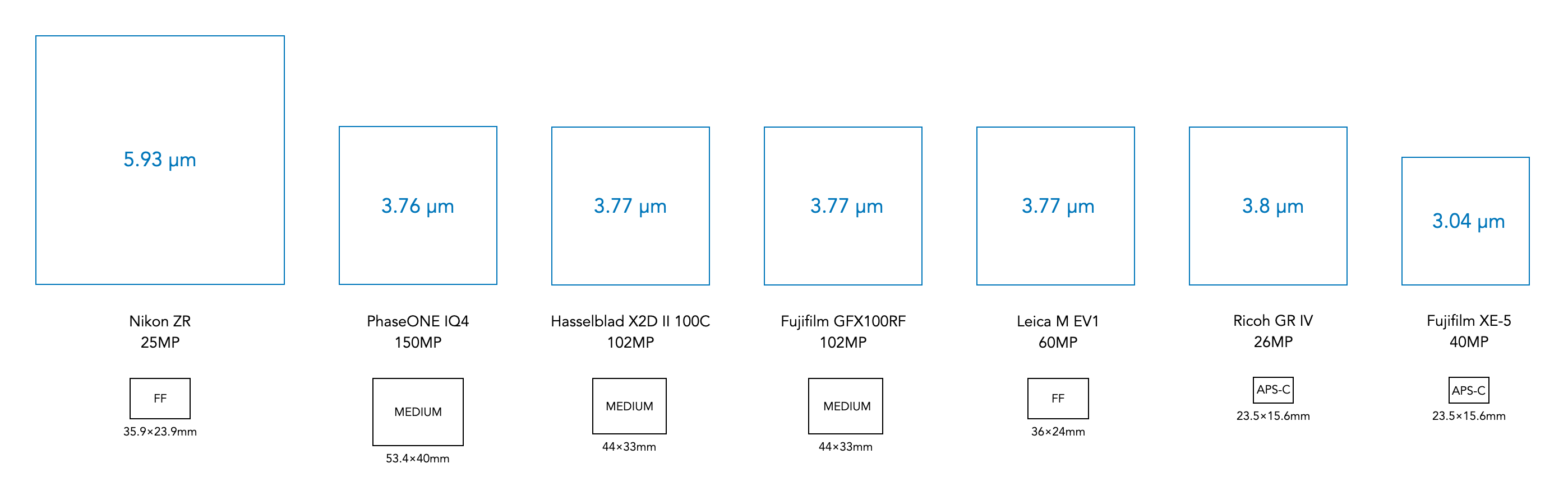
Advertising has never made mention of the fact that as more photosites were squeezed into a sensor, they get smaller. There are also intrinsic limits to how small photosites can get. APS-C sensors seem to have maxed out at roughly 40MP, with photosites approximately 3.0×3.0µm in size, the same size as the diameter of spiders silk (to put that into context the average human hair is 70µm in diameter). Manufacturers could push APS-C sensors toward 60MP, but this faces significant engineering challenges. There would be issues with diffraction at wider apertures leading to image softening, higher noise at high ISO values, and limitations of lenses being able to resolve details. Some might even argue that 26 million photosites is too many for an APS-C sensor.
As it stands, most people don’t need a camera with any more than 24-26MPs, especially when some cameras are now incorporating pixel-shift high resolution modes to facilitate high resolution images. For example the Fujifilm X-T5 features a Pixel Shift Multi-Shot mode that produces 160MP-images by combining 20 RAW frames, using IBIS to shift the 40.2MP sensor. Improvements in the quality of pixels will only come about with innovative new sensor technologies, e.g. stacked sensors.
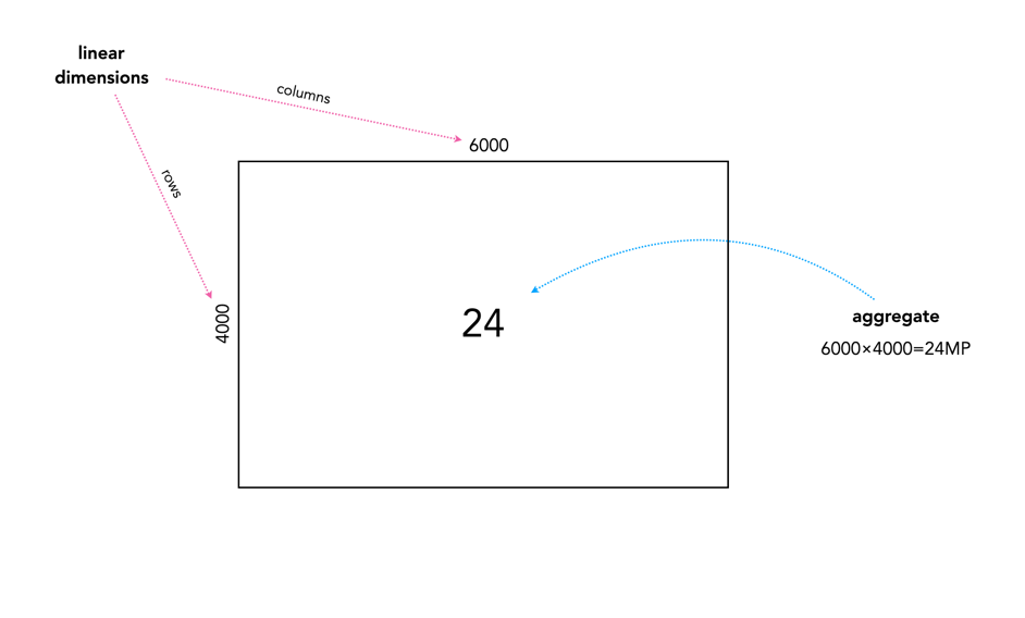
Note: Sensors have photosites (which have dimensions), while images have pixels (which are dimensionless).