the image histogram (iv) – shape

One of the most important characteristics of a histogram is its shape. A histogram’s shape offers a good indicator of an image’s ability to tolerate manipulation. A histogram shape can help elucidate the overall contrast in the image. For example a broad histogram usually reflects a scene with significant contrast, whereas a narrow histogram reflects less contrast, with an image which may appear dull or flat. As mentioned previously, some people believe an “ideal” histogram is one having a shape like a hill, mountain, or bell. The reality is that there are as many shapes as there are images. Remember, a histogram represents the pixels in an image, not their position. This means that it is possible to have a number of images that look very different, but have similar histograms.

The shape of a histogram is usually described in terms of simple shape features. These shape features are often described using geographical terms (because a histogram often reminds people of the profile view of a geographical feature): e.g. “hillock” or “mound”, which is a shallow, low feature, “hill” or “hump”, which is a feature rising higher than the surrounding areas, a “peak”, which is a feature with a distinctly top, a “valley”, which is a low area between two peaks, or a “plateau” which is a level region between other features. Features can either be distinct, i.e. recognizably different, or indistinct, i.e. not clearly defined, often blended with other features. These terms are often used when describing the shape of a particular histogram in detail.

Fig.1: A sample of feature shapes in a histogram

From the perspective of simplicity, however histogram shapes can be broadly classified into three basic categories (examples are shown in Fig.2):

  • Unimodal – A histogram where there is one distinct feature, typically a hump or peak, i.e. a good amount of an image’s pixels are associated with the feature. The feature can exist anywhere in the histogram. A good example of a unimodal histogram is the classic “bell-shaped” curve with a prominent ‘mound’ in the center and similar tapering to the left and right (e.g. Fig.2: ①).
  • Bimodal – A histogram where there are two distinct features. Bimodal features can exist as a number of varied shapes, for example the features could be very close, or at opposite ends of the histogram.
  • Multipeak – A histogram with many prominent features, sometimes referred to as multimodal. These histograms tend to differ vastly in their appearance. The peaks in a multipeak histogram can themselves be composed of unimodal or bimodal features.

These categories can can be used in combination with some qualifiers (numeric examples refer to Figure 2). For example a symmetric histogram, is a histogram where each half is the same. Conversely an asymmetric histogram is one which is not symmetric, typically skewed to one side. One can therefore have a unimodal, asymmetric histogram, e.g. ⑥ which shows a classic “J” shape. Bimodal histograms can also be asymmetric (⑪) or symmetric (⑬).

Fig.2: Core categories of histograms: unimodal, bimodal, multi-peak and other.

Histograms can also be qualified as being indistinct, meaning that it is hard to categorize it as any one shape. In ㉓ there is a peak to the right end of the histogram, however the major of the pixels are distributed in the uniform plateau to the right. Sometimes histogram shapes can also be quite uniform, with no distinct groups of pixels, such as in example ㉒ (in reality though these images are quite rare). It it also possible that the histogram exhibits quite a random pattern, which might only indicate quite a complex scene.

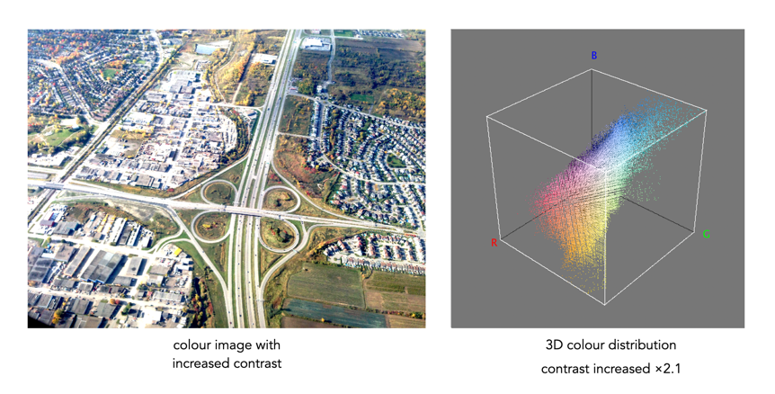
But a histogram’s shape is just its shape. To interpet a histogram requires understanding the shape in context to the contents of the scene within the image. For example, one cannot determine an image is too dark from a left-skewed unimodal histogram without knowledge of what the scene entails. Figure 3 shows some sample colour images and their corresponding histograms, illustrating the variation existing in histograms.

Fig.3: Various colour images and their corresponding intensity histograms

the image histogram (iii) – useful information

Some people think that the histogram is some sort of panacea for digital photography, a means of deciding whether an image is “perfect” enough. Others tend to disregard the statistical response it provides completely. This leads us to question what useful information is there in a histogram, and how we go about interpreting it.

A plethora of information

A histogram maps the brightness or intensity of every pixel in an image. But what does this information tell us? One of the main roles of a histogram is to provide information on the tonal distributions in an image. This is useful to help determine if there is something askew with the visual appearance of an image. Histograms can be viewed live/in-camera, for the purpose of determining whether or not an image has been corrected exposed, or used during post-processing to fix aesthetic inadequacies. Aesthetic deficiencies can occur during the acquisition process, or can be intrinsic to the image itself, e.g. faded vintage photographs. Examples of deficiencies include such things as blown highlights, or lack of contrast.

A histogram can tell us many differing things about how intensities are distributed throughout the image. Figure 1 shows an example of a colour image, photograph taken in Bergen, Norway, its associated grayscale image and histograms. The histogram spans the entire range of intensity values. Midtones comprise 66% of pixels in the image, with the majority tiered towards the lighter midtone values (the largest hump in the histogram). Shadow pixels comprise only 7% of the whole image, and are actually associated with shaded regions in the image. Highlights relate to regions like the white building on the left, and some of the clouds. There are very few pure white, the exception being the shopfront signs. Some of the major features in the histogram are indicated in the image.

Fig.1: A colour image and its histograms

There is no perfect histogram

Before we get into the nitty-gritty, there is one thing that should be made clear. Sometimes there are infographics on the internet that tout the myth of a “perfect” or “ideal” histogram. The reality is that such infographics are very misleading. There is no such thing as a perfect histogram. The notion of the ideal histogram is one that is shaped like a “bell”, but there is no reason why the distribution of intensities should be that even. Here is the usual description of an ideal image: “An ideal image has a histogram which has a centred hill type shape, with no obvious skew, and a form that is spread across the entire histogram (and without clipping)”.

Fig.2: A bell-shaped curve

But a scene may be naturally darker or lighter rather than midtones found in a bell-shaped histogram. Photographs taken in the latter part of the day will be naturally darker, as will photographs of dark objects. Conversely, a photograph of a snowy scene will skew to the right. Consider the picture of the Toronto skyline taken at night shown in Figure 3. Obviously the histogram doesn’t come close to being “perfect”, but the majority of the scene is dark – not unusual for a dark scene, and hence the histogram is representative of this. In this case the low-key histogram is ideal.

Fig.3: A dark image with a skewed histogram

Interpreting a histogram

Interpreting a histogram usually involves examining the size and uniformity of the distribution of intensities in the image. The first thing to do is to look at the overall curve of the histogram to get some idea about its shape characteristics. The curve visually communicates the number of pixels in any one particular intensity.

First, check for any noticeable peaks, dips, or plateaus. For example peaks generally indicate a large number of pixels of a certain intensity range within the image. Plateaus indicate a uniform distribution of intensities. Check to see if the histogram skewed to the left or right. A left-skewed histogram might indicate underexposure, the scene itself being dark (e.g. a night scene), or containing dark objects. A right-skewed histogram may indicate overexposure, or a scene full of white objects. A centred histogram may indicate a well-exposed image, because it is full of mid-tones. A small, uniform hill may indicate a lack of contrast.

Next look at the edges of the histogram. A histogram with peaks that are placed against either edge of the histogram may indicate some loss of information, a phenomena known as clipping. For example if clipping occurs on the right side, something known as highlight clipping, the image may be overexposed in some areas. This is a common occurrence in semi-bright overcast days, where the clouds can become blown-out. But of course this is relative to the scene content of the image. As well as shape, the histogram shows how pixels are groups into tonal regions, i.e. the highlights, shadows, and midtones.

Consider the example shown below in Figure 4. Some might interpret this as somewhat of an “ideal” histogram. Most of the pixels appear in the midtones region of the histogram, with no great amount of blacks below 17, nor whites above 211. This is a well-formed image, except that it lacks some contrast. Stretching the histogram over the entire range of 0-255 could help improve the contrast.

Fig.4: An ideal image with a central “hump” (but lacking some contrast)

Now consider a second example. This picture in Figure 5 is of a corner grocery store in Montreal and has a histogram with a multipeak shape. The three distinct features almost fit into the three tonal regions: the shadows (dark blue regions, and empty dark space to the right of the building), the midtones (e.g. the road), and the highlights (the light upper brick portion of the building). There is nothing intrinsically wrong with this histogram, as it accurately represents the scene in the image.

Fig.4: An ideal image with multiple peaks in the histogram

Remember, if the image looks okay from a visual perspective, don’t second-guess minor disturbances in the histogram.

Next: More on interpretation – histogram shapes.

Why are there no 3D colour histograms?

Some people probably wonder why there aren’t any 3D colour histograms. I mean if a colour image is comprised of red, green, and blue components, why not provide those in a combined manner rather than separate 2D histograms or a single 2D histogram with the R,G,B overlaid? Well, it’s not that simple.

A 2D histogram has 256 pieces of information (grayscale). A 24-bit colour image contains 2563 colours in it – that’s 16,777,216 pieces of information. So a three-dimensional “histogram” would contain the same number of elements. Well, it’s not really a histogram, more of a 3D representation of the diversity of colours in the image. Consider the example shown in Figure 1. The sample image contains 428,763 unique colours, representing just 2.5% of all available colours. Two different views of the colour cube (rotated) show the dispersion of colours. Both show the vastness of the 3D space, and conversely the sparsity of the image colour information.

Figure 1: A colour image and 3D colour distribution cubes shown at different angles

It is extremely hard to create a true 3D histogram. A true 3D histogram would have a count of the number of pixels with a particular RGB triplet at every point. For example, how many times does the colour (23,157,87) occur? It’s hard to visualize this in a 3D sense, because unlike the 2D histogram which displays frequency as the number of occurrences of each grayscale intensity, the same is not possible in 3D. Well it is, kind-of.

In a 3D histogram which already uses the three dimensions to represent R, G, and B, there would have to be a fourth dimension to hold the number of times a colour occurs. To obtain a true 3D histogram, we would have to group the colours into “cells” which are essentially clusters representing similar colours. An example of the frequency-weighted histogram with for the image in Figure 2, using 500 cells, is shown in Figure 2. You can see that while in the colour distribution cube in Figure 1 shows a large band of reds, because these colours exist in the image, the frequency weighted histogram shows that objects with red colours actually comprise a small number of pixels in the image.

Figure 2: The frequency-distributed histogram of the image in Fig.1

The bigger problem is that it is quite hard to visualize a 3D anything and actively manipulate it. There are very few tools for this. Theoretically it makes sense to deal with 3D data in 3D. The application ImageJ (Fiji) does offer an add-on called Color Inspector 3D, which facilitates viewing and manipulating an image in 3D, in a number of differing colour spaces. Consider another example, shown in Figure 3. The aerial image, taken above Montreal lacks contrast. From the example shown, you can see that the colour image takes up quite a thin band of colours, almost on the black-white diagonal (it has 186,322 uniques colours).

Figure 3: Another sample colour image and its 3D colour distribution cube

Using the contrast tool provided in ImageJ, it is possible to manipulate the contrast in 3D. Here we have increased the contrast by 2.1 times. You can easily see the result in Figure 4. difference working in 3D makes. This is something that is much harder to do in two dimensions, manipulating each colour independently.

Figure 4: Increasing contrast via the 3D cube

Another example of increasing colour saturation 2 times, and the associated 3D colour distribution is shown in Figure 5. The Color Inspector 3D also allows viewing and manipulating the image in other colour spaces such as HSB and CieLab. For example in HSB the true effect of manipulating saturation can be gauged. The downside is that it does not actually process the full-resolution image, but rather one reduced in size, largely because I imagine it can’t handle the size of the image, and allow manipulation in real-time.

Figure 5: Increasing saturation via the 3D cube

the image histogram (ii) – grayscale vs colour

In terms of image processing there are two basic types of histogram: (i) colour, and (ii) intensity (or luminance/grayscale) histograms. Figure 1 shows a colour image (an aerial shot of Montreal), and its associated RGB and intensity histograms. Colour histograms are essentially RGB histograms, typically represented by three separate histograms, one for each of the components – Red, Green, and Blue. The three R,G,B histograms are sometimes shown in one mixed histogram with all three R,G,B, components overlaid with one another (sometimes including an intensity histogram).

Fig.1: Colour and grayscale histograms

Both RGB and intensity histograms contain the same basic information – the distribution of values. The difference lies in what the values represent. In an intensity histogram, the values represent the intensity values in a grayscale image (typically 0 to 255). In an RGB histogram, divided into individual R, G, B histograms, each colour channel is just a graph of the frequencies of each of the RGB component values of each pixel.

An example is shown in Figure 2. Here a single pixel is extracted from an image. The RGB triplet for the pixel is (230,154,182) i.e. it has a red value of 230, a green value of 154, and a blue value of 182. Each value is counted in its respective bin in the associated component histogram. So red value 230 is counted in the bin marked as “230” in the red histogram. The three R,G, B histograms are visually no different than an intensity histogram. The individual R, G, and B histograms do not represent distributions of colours, but merely distributions of components – for that you need a 3D histogram (see bottom).

Fig.2: How an RGB histogram works: From single RGB pixel to RGB component histograms

Applications portray colour histograms in many different forms. Figure 3 shows the RGB histograms from three differing applications: Apple Photos, ImageJ, and ImageMagick. Apple Photos provides the user with the option of showing the luminance histogram, the mixed RGB, or the individual R, G, B histograms. The combined histogram shows all the overlaid R, G, B histograms, and a gray region showing where all three overlap. ImageJ shows the three components in separate histograms, and ImageMagick provides an option for their combined or separate. Note that some histograms (ImageMagick) seem a little “compressed”, because of the chosen x-scale.

Fig.3: How RGB histograms are depicted in applications

One thing you may notice when comparing intensity and RGB histograms is that the intensity histogram is very similar to the green channel or the RGB image (see Figure 4). The human eye is more sensitive to green light than red or blue light. Typically the green intensity levels within an image are most representative of the brightness distribution of the colour image.

Fig.4: The RGB-green histogram verus intensity histogram

An intensity image is normally created from an RGB image by converting each pixel so that it represents a value based on a weighted average of the three colours at that pixel. This weighting assumes that green represents 59% of the perceived intensity, while the red and blue channels account for just 30% and 11%, respectively. Here is the actual formula used:

gray = 0.299R + 0.587G + 0.114B

Once you have a grayscale image, it can be used to derive an intensity histogram. Figure 5 illustrates how a grayscale image is created from an RGB image using this formula.

Fig.5: Deriving a grayscale image from an RGB image

Honestly there isn’t really that much useful data in RGB histograms, although they seem to be very common in image manipulation applications, and digital cameras. The problem lies with the notion of the RGB colour space. It is a space in which chrominance and luminance are coupled together, and as such it is difficult to manipulate any one of the channels without causing shifts in colour. Typically, applications that allow manipulation of the histogram do so by first converting the image to a decoupled colour space such as HSB (Hue-Saturation-Brightness), where the brightness can be manipulated independently of the colour information.

A Note on 3D RGB: Although it would be somewhat useful, there are very few applications that provide a 3D histogram, constructed from the R, G, and B information. One reason is that these 3D matrices could be very sparse. Instead of three 2D histograms, each with 256 pieces of information, there is now a 3D histogram with 2563 or 16,777,216 pieces of information. The other reason is that 3D histograms are hard to visualize.

the image histogram (i) – what is it?

An image is really just a collection of pixels of differing intensities, regardless of whether it is a grayscale (achromatic) or colour image. Exploring the pixels collectively helps provide an insight into the statistical attributes of an image. One way of doing this is by means of a histogram, which represents statistical information in a visual format. Using a histogram it is easy to determine whether there are issues with an image, such as over-exposure. In fact histograms are so useful that most digital cameras offer some form of real-time histogram in order to prevent poorly exposed photographs. Histograms can also be used in post-processing situations to improve the aesthetic appeal of an image.

Fig.1: A colour image with its intensity histogram overlaid.

A histogram is simply a frequency distribution, represented in the form of a graph. An image histogram, sometimes called an intensity histogram, describes the frequency of intensity (brightness) values that occur in an image. Sometimes as in Figure 1, the histogram is represented as a bar graph, while other times it appears as a line graph. The graph typically has “brightness” on the horizontal axis, and “number of pixels” on the vertical axis. The “brightness” scale describes a series of values in a linear scale from 0, which represents black, to some value N, which represents white.

Fig.2: A grayscale image and its histogram.

A image histogram, H, contains N bins, with each bin containing a value representing the number of times an intensity value occurs in an image. So a histogram for a typical 8-bit grayscale image with 256 gray levels would have N=256 bins. Each bin in the histogram, H[i] represents the number of pixels in the image with intensity i. Therefore H[0] is the number of pixels with intensity 0 (black), H[1] the number of pixels with intensity 1, and so forth until H[255] which is the number of pixels with the maximum intensity value, 255 (i.e. white).

A histogram can be used to explore the overall information in an image. It provides a visual characterization of the intensities, but does not confer any spatial information, i.e. how the pixels physically relate to one another in the image. This is normal because the main function of a histogram is to represent statistical information in a compact form. The frequency data can be used to calculate the minimum and maximum intensity values, the mean, and even the median.

This series will look at the various types of histograms, how they can be used to produce better pictures, and how they can be manipulated to improve the aesthetics of an image.

Image histograms tell a story

The simplest data about an image it that contained within its histogram, or rather the distribution of pixel intensities. In an 8-bit grayscale image, this results in a 256-bin histogram which tells a story about how the pixels are distributed within the image. Most digital cameras also have some form of colour histogram which can be used to determine distribution of colours in an image.  This lets the photographer determine whether the photograph is over- under- or correctly exposed.  A correctly exposed photograph will have a fairly uniform histogram, whereas an under-exposed one has a bias towards darker tones, and an over-exposed one will have a bias towards brighter  tones.

This by no means means that a histogram that has two distinct modes does not represent a good image. As long as the histogram is well distributed between the lower and upper limits of the colour space. Consider the image below:

From an aesthetic perspective, this does not seem like a bad looking image. Its histogram somewhat collaborates this:

In fact there is limited scope for enhancement here. Application of  contrast-stretching or histogram equalization will increase its aesthetic appeal marginally. One of the properties of an image that a histogram helps identify is contrast, or dynamic range. On the other end of the spectrum, consider this image which has a narrow dynamic range.

The histogram clearly shows the lack of range in the image.

Stretching the histogram to either end of the spectrum increases the contrast of the image. The result is shown below.

It has a broader dynamic range, and a greater contrast of features within the image.