The funny thing about the photosites on a sensor is that they are mostly designed to pick up one colour, due to the specific colour filter associated with with photosite. Therefore a normal sensor does not have photosites which contain full RGB information.
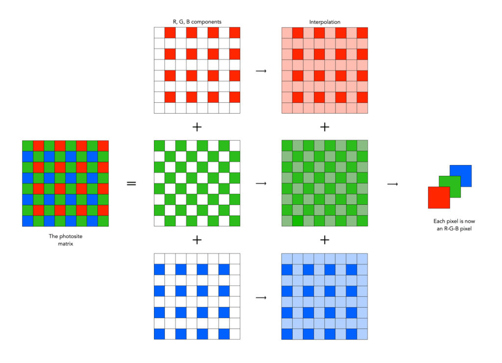
To create an image from a photosite matrix it is first necessary to perform a task called demosaicing (or demosaiking, or debayering). Demosaicing separates the red, green, and blue elements of the Bayer image into three distinct R, G, and B components. Note a colouring filtering mechanism other than Bayer may be used. The problem is that each of these layers is sparse – the green layer contains 50% green pixels, and the remainder are empty. The red and blue layers only contain 25% of red and blue pixels respectively. Values for the empty pixels are then determined using some form of interpolation algorithm. The result is an RGB image containing three layers representing red, green and blue components for each pixel in the image.
A basic demosaicing process
There are a myriad of differing interpolation algorithms, some which may be specific to certain manufacturers (and potentially proprietary). Some are quite simple, such as bilinear interpolation, while others like bicubic interpolation, spline interpolation, and Lanczos resampling are more complex. These methods produce reasonable results in homogeneous regions of an image, but can be susceptible to artifacts near edges. This leads to more sophisticated algorithms such as Adaptive Homogeneity-Directed, and Aliasing Minimization and Zipper Elimination (AMaZE).
An example of bilinear interpolation is shown in the figure below (note that no cameras actually use bilinear interpolation for demosaicing, but it offers a simple example to show what happens). For example extracting the red component from the photosite matrix leaves a lot of pixels with no red information. These empty reds are interpolated from existing red information in the following manner: where there was previously a green pixel, red is interpolated as the average of the two neighbouring red pixels; and where there was previously a blue pixel, red is interpolated as the average of the four (diagonal) neighbouring red pixels. This way the “empty” pixels in the red layer are interpolated. In the green layer every empty pixel is simply the average of the neighbouring four green pixels. The blue layer is similar to the red layer.
One of the simplest interpolation algorithms, bilinear interpolation.
❂ The only camera sensors that don’t use this principle are the Foveon-type sensors which have three separate layers of photodetectors (R,G,B). So stacked the sensor creates a full-colour pixel when processed, without the need for demosaicing. Sigma has been working on a full-frame Foveon sensor for years, but there are a number of issues still to be dealt with including colour accuracy.
Some of the most interesting vintage lenses are the sub-f/1.2 lenses, of which there are very few. In the 1950s Japanese lens makers wanted to push the envelope, racing to construct the fastest lenses possible. There were four contenders: the Zunow 50mm f/1.1, the Nippon Kogaku’s Nikkor-N.C 50mm f/1.1, Konishiroku (Konica’s predecessor) Hexanon 60mm f/1.2 and the Fujinon 50mm f1.2 LTM. This spurned research which led to the development of the Canon 50mm f/0.95 (1961), which at the time was the largest aperture of any cameras lens in the world. The other, which did not appear until 1976 was the Leitz (Canada) Noctilux-M 50mm f/1.0.
(Note that these lenses were made for 35mm rangefinder cameras.)
Why were these lenses developed?
The most obvious reason was the race to produce fast lenses. An article in the February 1956 issue of Popular Photography sheds more light on the issue. The article, titled “Meet the Zunow f/1.1” [1], by Norman Rothschild, described the virtues of the Zunow lens (more on that below), and concluded with one of the reasons these lenses were of interest, namely that it opened up new areas for the “available-light man”, i.e. the person who wanted to use only natural light, especially with slow colour films. This makes sense, as Kodachrome had an ASA speed of 10, and Type A’s speed was ASA 16. Even Kodachrome II released in 1961 only had a speed of 25 ISO. Conversely, black and white film of the period was much faster: Kodak Super-XX was 200 ISO, and Ilford FP3 was 125 ISO. Ilford HPS, introduced in 1954 pushed the ISO to 800. The newer Ektachrome and Anscochrome colour films were rated at ASA 32. In the patent for the Zunow f/1.1 lens [3], the authors claimed that objectives with apertures wider than f/1.4 were in more demand. In reality, the race to make even faster lenses was little different to the race to get to the moon.
Zunow 50mm f/1.1
The first of the sub-5/1.2 lenses was the Zunow 50mm f/1.1. Teikoku Kōgaku Kenkyūjo was founded by Suzuki Sakuta circa 1930 and worked for other companies grinding lenses. The company started working on fast lens around 1948, with the first prototypes completed in 1950, and the 50mm f/1.1 Zunow released in 1953. It made a number of lenses for rangefinder cameras, including slower 50mm lenses in f/1.3, and f/1.9, a f/1.7 35mm, and a 100mm f/2 lenses. In 1956 it became the Zunow Kōgaku Kōgyō K.K., or Zunow Optical Industry Co., Ltd., but closed its doors in early 1961. During the last years the company designed a couple of camera’s including a prototype of a Leica copy, the Teica, and the Zunow SLR, the first 35mm SLR camera with auto diaphragm, instant-return mirror, and bayonet mount interchangeable lenses (only about 500 were ever produced).
The Zunow 50mm f/1.1 was derived from the Sonnar-type f/1.5 lens. The patent for the Zunow f/1.1 lens [3] describes the lens as “an improved photographic objective suited for use with a camera that takes 36×24mm pictures”. Many of these fast lenses were actually manufactured for the cine industry. For example the company produced Zunow-Elmo Cine f/1.1 lenses for D-mount in 38mm and 6.5mm (and these lenses are reasonably priced, circa US$500, however not very useful for 35mm). The Zunow 50mm f/1.1 is today a vary rare lens. Sales are are US$5-10K depending on condition. The price for this lens in 1956 was US$450.
1953 – Zunow f/1.1 5cm, Leica M39 mount/Nikon S, 9 elements in 5 groups.
1955 – Zunow f/1.1 50mm, Leica M39 mount/Nikon S, 8 elements in 5 groups.
Nikkor-N 50mm f/1.1
Hot on the heals of Zunow was the Nikkor-N 5cm f/1.1 developed by Nippon Kogaku. Introduced in 1956, it was the second sub-f/1.2 lens produced. The lens was designed by Saburo Murakami, who received a patent for it in 1958 [5]. While the Zunow was an extension of the Sonnar-type lens, the Nikkor lens was of a gaussian type. It was also made using an optical glass made using the rare earth element Lanthanum in three of its optical elements. The lens was made in three differing mounts: the original internal Nikon mount (for use on Nikon S2, SP/S3 cameras), the external Nikon mount, and the Leica M39 mount. The original lens mount was an internal mount, and the heavy weight of the lens (425g) could damage the focusing mount, so it was redesigned in 1959 with an external mount. The lens had a gigantic lens hood with cut-outs for setting the focus with the rangefinder through the viewfinder.
1956 – Nikon Nikkor-N[.C] 50mm f/1.1, Leica screw mount/Nikon S, 9 elements in 6 groups (Nikon, 1200 units; M39, 300 units)
1959 – Nikon Nikkor-N 50mm f/1.1, Leica screw mount/Nikon S, 9 elements in 6 groups (1800 units)
A 1959 price list shows that this lens sold for US$299.50. Today the price of this lens is anywhere in the range $5-10K. Too few were manufactured to make this lens the least bit affordable. Nippon Kogaku also supposedly developed an experimental f/1.0 lens for the Nikon S, but it never went into production.
Canon 50mm f/0.95
In August 1961, Canon released the 50mm f/0.95, designed as a standard lens for the Canon 7 rangefinder camera. It was the world’s fastest lens. The Canon f/0.95 was often advertised attached to the Model 7 camera – the Canon “dream” lens. The advertising generally touted the fact that it was “the world’s fastest lens, four times brighter than the human eye” (how this could be measured is questionable). It is Gauss type lens with 7 elements in 5 groups. The lens was so large on the Canon 7 that it obscured a good part of the view in the bottom right-hand corner of the viewfinder, and partially obscured the field-of-view.
In a 1970 Canon price list, the 50mm f/0.95 rangefinder lens sold for $320, with the f/1.2 at $220. To put this into context, $320 in 1970 is worth about $2320 today, and a Canon 7 with a f/0.95 lens in average condition sells for around this value. Lenses in mint condition are valued at around $5K.
The verdict?
So why did these lenses not catch on? Cost for one. While f/1.2 lenses were expensive, faster lenses were even more expensive. For specialist applications, the development of these lenses likely made sense, but for the average photographer likely not. There were a number of articles circa 1950 in magazines like Poplular Photography which seemed to downplay their value, which likely contributed to their decline. It is notable that by the the early 1960s, Nikon stopped advertising its 50mm f/1.1 lens, and never produced another sub-f/1.2 lens. By the late 1960s even Canon had ceased production of the f/0.95.
There were probably more sub f/1.2 lenses created for non-photographic applications, in many different focal lengths. For example x-ray machines (Leitz 50mm f/0.75), D-mount film cameras (e.g. Kern Switar 13mm f/0.9), C-mount for film, medical and scientific imaging (e.g. Angenieux 35mm f/0.95), and aerial photography lenses (e.g. Zeiss Planar 50mm f/0.7). Not until recently have super-fast lenses once again appeared, likely because they are technologically better lenses, made much cheaper than they ever could have been in the 1950s and 60s.
References:
Norman Rothschild, “Meet the Zunow f/1.1”, Popular Photography, pp.126/128, February (1956)
Kogoro Yamada, “Japanese photographic objectives for use with 35mm cameras”, Photographic Science and Engineering 2(1), p.6-13 (1958)
U.S. Patent 2,715,354, Sakuta Suzuki et al., “Photographic Objective with Wide Relative Aperture”, August 16, (1955)
Hagiya Takeshi, Zunō kamera tanjō: Sengo kokusan kamera jū monogatari (The birth of the Zunow camera: Ten stories of postwar Japanese camera makers) Japanese only (1999)
U.S. Patent 2,828,671, “Wide Aperture Photographic Objectives”, April 1, 1958.
Everything in modern digital photography seems to hark back to analogue 35mm. The concept of “full-frame” only exists because a full frame sensor is equivalent in size to the 24×36mm frame of 35mm film (which was only called 35mm because that was the width of the film). If we didn’t have this association, there would be no crop-sensor. Most early films for cameras were quite large format – introduced in 1899, 116 format film was 70mm wide. This was followed in 1901 by 120 (60mm), 127 (40mm) in 1912, and then 620 (60mm) in 1931. So there were certainly many film format options. So why did 35mm become the standard?
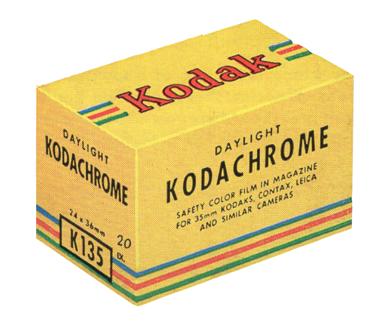
In all likelihood, 35mm became the gold standard because of how widely available 35mm film was in the motion picture industry – it had been around since 1889 when Thomas Edison’s assistant, William Kennedy Dickson simply split 70mm Eastman Kodak film in half. (I have discussed the origins of 35mm film in a previous post). Kodak introduced the standard 135 film in 1934, and was designed for making static pictures (rather than film) with the actual exposure frames being 36mm wide, and 24mm high, giving it a 3:2 ratio. In the 1930s, Leica brochures expounded the fact that the film used in their cameras was “…the standard 35mm cinema film stock, obtainable all over the world.“
A standard Leica with a 50mm f/3.5 ELMAR lens
There was much hype in the 1930s about the cameras that were termed “minicams”, or “candid cameras”, in effect cameras that used 35mm film. By the mid 1930s, Leica had been producing 35mm cameras for over a decade. A 1936 Fortune Magazine article titled “The U.S. Minicam Boom” described the Leica as a camera which “took thirty-six pictures the size of the special-delivery stamp on a roll of movie film.” There were those who did not think the miniature camera would survive, seeing their use as a form of candid camera craze. Take for example the closing argument of Thomas Uzzell, who wrote the negative perspective of a 1937 article “Will the Miniature Survive the Candid Camera Craze?” [1]:
“The little German optical jewels you carry in your (sagging) coat pockets make many experimental exposures expensive (though perhaps they would do better if they carefully made one good one!). Their shorter focal lengths make the ultra-fast exposures more practical (how many pictures are actually taken at these ultra speeds!). You can hop about quickly, minnie in hand, and take photos of children and babies at play with all the detail that “makes a picture pulse with naturalness and life” (though good pictures have never been taken by anyone hoping about). … I claim there is just one thing they cannot do, and apparently are never going to be able to do. They can’t make clear pictures.”
Uzzell claimed the art of the miniature was the art of the fuzzy picture. His challenger, Homer Jensen on the other hand described the inherent merits of 35mm over larger format cameras, namely that one could “…take pictures under the most unfavourable conditions, indoors and outdoors.”. Some people disliked the minicam because it made it too easy to take pictures (like anyone could take pictures).
One of the reasons 35mm was so successful was the small size of the camera itself. Their lightweight nature made them easy to carry, taking up very little room. This made them popular with both causal photographers and professionals such as photojournalists where the use of bulky equipment would be prohibitive. Another reason was the 35mm camera’s ability to work in existing light conditions. This was an affect of having ultra-fast lenses, something the larger format cameras could not practically achieve. The shorter focal lengths of 35mm cameras also allowed for greater depth-of-field at wide lens apertures. The inaugural issue of Popular Photography in 1937 described the advantages of using miniatures to capture fast action [4].
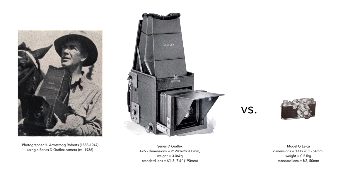
A large format Graflex camera versus a Leica “minicam”.
Large format cameras on the other hand, were sometimes referred to as “Big Berthas” due to their size [4]. The Series D Graflex, a quintessential 4×5″ press camera of the 1930s weighed 3.06kg, compared with the Leica G, which was one-sixth its weight, and roughly 1/30th its size. In a Graflex brochure from 1936, photographer H. Armstrong Roberts recalls a recent 14,000 mile journey where he took 3000 negatives using his Graflex camera, stating that “Certain I am that no other camera could have achieved the results which I have obtained with the GRAFLEX.”
In 1935, another event foreshadowed the success of 35mm photography – Kodak’s introduction of Kodachrome colour film, followed shortly afterwards by Agfa’s Agfacolor Neu. This may have persuaded many a professional photographer to move to 35mm. Indeed, by 1938, H. Armstrong Roberts was also shooting in colour using a Zeiss Contaflex with a 50mm f/2 Sonnar lens [5] (so much for his belief in large format). The onset of WW2 brought a halt to the first minicam boom, but it was not the end of the story. By the early 1950s, the minicam was on the cusp of greatness, soon to become the standard means of taking photographs. More articles started to appear in photography magazines, enunciating the virtues of 35mm [3].
There are many reasons 35mm film became the format of choice.
Kodak’s 135 film single-use cartridge allowed for daylight loading. Prior to this 35mm film had to be loaded onto reusable cassettes in the darkroom.
The physical format of 35mm film made it very user friendly. The film is contained in a metal canister that reduces the risk of light leaks, and is easy to handle. Loading/unloading film is both intuitive, quick and easy. It’s compact size made it much easier to handle than larger format film.
35mm also allowed for more exposures per roll than typical large format films. The norm is 24 or 36 exposures. This provided a great deal of flexibility in the amount of shots that could be taken, because 35mm film was easier and cheaper to develop.
In the hey-day of film photography there was a huge selection of film types – B&W, colour, infrared, and slide.
Of course there were also some limitations, but these mostly centre on the fact that 35mm film was considered to have less resolving power than medium-format film – great for “snapshots”, but anyone that required large prints needed a large film format to avoid grainy prints.
The invention of the Leica started a new era in photography, spurned on by the introduction of Kodak’s 135 film. Post WW2, 35mm film spearheaded the photographic revolution of the 1950s. It became the format used by amateurs, hobbyists, and professionals alike. 35mm photography allowed for a light, yet flexible kit, which was ideal for the travelling amateur photographer of the 1960s.
Further reading:
Uzzell, Thomas, H., “Will the Miniature Survive the Candid Camera Craze? – No”, PopularPhotography, 1(4), pp. 32,66 (1937)
Jensen, Homer, “Will the Miniature Survive the Candid Camera Craze? – Yes”, PopularPhotography, 1(4), pp. 33,84 (1937)
“35mm: The camera and how to use it”, Popular Photography, pp.50-54,118, November (1951)
Witwer, Stan, “Fast Action with a Miniature”, Popular Photography, 1(1) pp.19-20,66 (1937)
“Taking the May Cover in Color”, Popular Photography, 2(5) pp.54 (1938)
The highest “native” resolution camera available today is the Phase One FX IQ4 medium format camera at 150MP. Higher than that there is the Hasselblad H6D-400C at 400MP, but it uses pixel-shift image capture. Next in line is the medium format Fujifilm GFX 100/100S at 102 MP. In fact we don’t get to full-frame sensors until we hit the Sony A7R IV, at a tiny 61MP. Crazy right? The question is how useful are these sensors for the photographer? The answer is not straightforward. For some photographic professionals these large sensors make inherent sense. For the average casual photographer, they likely don’t.
People who don’t photograph a lot tend to be somewhat bamboozled by megapixels, like more is better. But more megapixels does not mean a better image. Here are some things to consider when thinking about when considering megapixels.
Sensor size
There is a point when it becomes hard to cram any more photosites into a particular sensor – they just become too small. For example the upper bound with APC-S sensors seems to be around 33MP, with full-frame it seems to be around 60MP. Put too many photosites on a sensor and the density of the photosites increases, as the size of the photosites decreases. The smaller the photosite, the harder it is for it to collect light. For example Fuji APS-C cameras seem to tap out at around 26MP – the X-T30 has a photosite pitch of 3.75µm. Note that Fuji’s leap to a larger number of megapixels also means a leap to a larger sensor – the medium format sensor with a sensor size of 44×33mm. Compared to the APS-C sensor (23.5×15.6mm), the medium format sensor is nearly four times the size. A 51MP medium format sensor has photosites which are 5.33µm in size, or 1.42 times of size of the 26MP APS-C sensor.
The verdict? Squeezing more photosites onto the same size sensor does increase resolution, but sometimes at the expense of how light is acquired by the sensor.
Image and linear resolution
Sensors are made up of photosites that acquire the data used to make image pixels. The image resolution of an image describes the number of pixels used to construct an image. For example a 16MP sensor with a 3:2 aspect ratio has an image resolution of 4899×3266 pixels – the dimensions are sometimes termed the linear resolution. To obtain twice the image resolution we need a 64MP sensor, rather than a 32MP sensor. A 32MP sensor has 6928×4619 photosites, which results in a 1.4 times increase in the linear resolution of the image. The pixel count has doubled, but the linear resolution has not. Upgrading from a 16MP sensor to a 24MP sensor means a ×1.5 increase in the pixel count, and a ×1.2 increase in linear resolution. The transition from 16MP to 64MP is a ×2 increase in linear resolution, and a ×4 increase in the number of pixels. That’s why the difference between 16MP and 24MP sensors is also dubious (see Figure 1).
Fig.1: Differentimage resolutions and megapixels within an APS-C sensor
To double the linear resolution of a 24MP sensor you need a 96MP sensor. So the 61MP sensor provides about double the linear resolution of a 16MP sensor, as the 102MP sensor doubles the 24MP sensor.
The verdict? Doubling the pixel count, i.e. image resolution, does not double the linear resolution.
Photosite size
When you have more photosites, you also have to ask what their physical size is. Squeezing 41 million photosites on the same size sensor as one which previously had 24 million pixels means that each pixel will be smaller, and that comes with its own baggage. Consider for instance the full-frame camera, the full-frame Leica M10-R, which has a 7864×5200 photosites (41MP) meaning the photosite size is roughly 4.59 microns. The full-frame 24MP Leica M-E has a photosite size of 5.97 microns, so 1.7 times the area. Large photosites allow more light to be captured, while smaller photosites gather less light, so when their low signal strength is transformed into a pixel, more noise is generated.
The verdict? From the perspective of photosite size, 24MP captured on a full-frame sensor will be better than 24MP on an APS-C sensor, which in turn is better than 24MP on a M43 sensor (theoretically anyways).
Optics
Comparing the quality of a 16MP lens to a 24MP lens, we might determine that the quality, and sharpness of the lens is more important than the number of pixels. In fact too many people place an emphasis on the number of pixels and forget about the fact that light has to pass through a lens before it is captured by the sensor and converted into an image. Many high-end cameras already provide an in-camera means of generating a high-resolution images, often four times the actual image resolution – so why pay more for more megapixels? Is a 50MP full-frame sensor any good without optically perfect (or near-perfect) lenses? Likely not.
The verdict? Good quality lenses are just as important as more megapixels.
File size
People tend to forget that images have to be saved on memory cards (and post-processed). The greater the megapixels, the greater the resulting file size. A 24MP image stored as a 24-bit/pixel JPEG will be 3.4MB in size (at 1/20). As a 12-bit RAW the file size would be 34MB. A 51MP camera like the Fujifilm GFX 50S II would have a 7.3MB JPEG, and a 73MB 12-bit RAW. If the only format used is JPEG it’s probably, fine, but the minute you switch to RAW it will use way more storage.
The verdict? More megapixels = more megabytes.
Camera use
The most important thing to consider may be what the camera is being used for?
Website / social media photography – Full-width images for websites are optimal at around 2400×1600 (aka 4MP), blog-post images max. 1500 pixels in width (regardless of height), and inside content max 1500×1000. Large images can reduce website performance, and due to screen resolution won’t be visualized to their fullest capacity anyways.
Digital viewing – 4K televisions have roughly 3840×2160 = 8,294,400 pixels. Viewing photographs from a camera with a large spatial resolution will just mean they are down-sampled for viewing. Even the Apple Pro Display XDR only has 6016×3384=20MP view capacity (which is a lot).
Large prints – Doing large posters, for example 20×30″ requires a good amount of resolution if they are being printed at 300DPI, which is the nominal standard. So this needs about 54MP (check out the calculator). But you can get by with less resolution because few people view a poster at 100%.
Average prints – An 8×10″ print requires 2400×3000 = 7.2MP at 300DPI. A 26MP image will print maximum size 14×20″ at 300DPI (which is pretty good).
Video – Does not need high resolution, but rather 4K video at a descent frame rate.
The verdict? The megapixel amount really depends on the core photographic application.
Postscript
So where does that leave us? Pondering a lot of information, most of which the average photographer may not be that interested in. Selecting the appropriate megapixel size is really based on what a camera will be used for. If you commonly take landscape photographs that are used in large scale posters, then 61 or 102 megapixels is certainly not out of the ballpark. For the average photographer taking travel photos, or for someone taking images for the web, or book publishing, then 16MP (or 24MP at the higher end) is ample. That’s why smartphone cameras do so well at 12MP. High MP cameras are really made more for professionals. Nobody needs 61MP.
The overall erdict? Most photographers don’t need 61 megapixels. In reality anywhere between 16 and 24 megapixels is just fine.
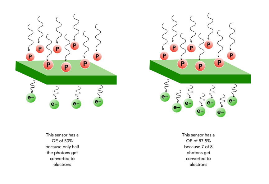
Not every photo that makes it through the lens ends up in a photosite. The efficiency with which photosites gather incoming light photons is called its quantum efficiency (QE). The ability to gather light is determined by many factors including the micro lenses, sensor structure, and photosite size. The QE value of a sensor is a fixed value that depends largely on the chip technology of the sensor manufacturer. The QE is averaged out over the entire sensor, and is expressed as the chance that a photon will be captured and converted to an electron.
Quantum efficiency (P = Photons per μm2, e = electrons)
The QE is a fixed value and is dependent on a sensor manufacturers design choices. The QE is averaged out over the entire sensor. A sensor with an 85% QE would produce 85 electrons of signal if it were exposed to 100 photons. There is no way to effect the QE of a sensor, i.e. you can’t change things by changing the ISO.
The QE is typically 30-55% meaning 30-55% of the photons that fall on any given photosite are converted to electrons. (front illuminated sensors). In back illuminated sensors, like those typically found on smartphones, the QE is approximately 85%. The website Photons to Photos has a list of sensor characteristics for a good number of cameras. For example the sensor in my Olympus OM-D E-M5 Mark II has a supposed QE of 60%. Trying to calculate the QE of a sensor in non-trivial.
We use the term “cropped sensor” only due to the desire to describe a sensor in terms of the 35mm standard. It is a relative term which compares two different types of sensor, but it isn’t really that meaningful. Knowing that a 24mm MFT lens “behaves” like a 48mm full-frame lens is pointless if you don’t understand how a 48mm lens behaves on a full-frame camera. All sensors could be considered “full-frame” in the context of their environment, i.e. a MFT camera has a full-frame sensor as it relates to the MFT standard.
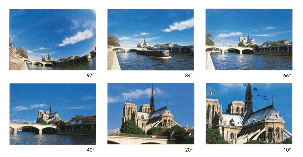
As mentioned in a previous post, the “35mm equivalence” is used to relate a crop-factor lens to its full-frame equivalent. The biggest problem with this is the amount of confusion it creates for novice photographers. Especially as focal lengths on lenses are always the same, yet the angle-of-view changes according to the sensor. However there is a solution to the problem, and that is to stop using the focal length to define a lens, and instead use AOV. This would allow people to pick a lens based on its angle-of view, both in degrees, but also from a descriptive point of view. For example, a wide angle lens in full-frame is 28mm – its equivalent in APS-C in 18mm, and MFT is 14mm. It would be easier just to label these by the AOV as “wide-74°”.
It would be easy to categorize lenses into six core groups based on horizontal AOV (diagonal AOV in []) :
Ultra-wide angle: 73-104° [84-114°]
Wide-angle: 54-73° [63-84°]
Normal (standard): 28-54° [34-63°]
Medium telephoto: 20-28° [24-34°]
Telephoto: 6-20° [8-24°]
Super-telephoto: 3-6° [4-8°]
Lenses could be advertised using a graphic to illustrate the AOV (horizontal) of the lens. This effectively removes the need to talk about focal length.
They are still loosely based on how AOV related to 35mm focal lengths. For example 63° relates to the AOV of a 35mm lens, however it no longer really relates to the focal length directly. A “normal-40°” lens would be 40° no matter the sensor size, even though the focal lengths would be different (see table below). The only lenses left out of this are fish-eye lenses, which in reality are not that common, and could be put into a specialty lens category, along with tilt-shift etc.
Instead of brochures containing focal lengths they could contain the AOV’s.
I know most lens manufacturers describe AOV using diagonal AOV, but this is actually more challenging for people to perceive, likely because looking through a camera we generally look at a scene from side-to-side, not corner-to-corner.
Lenses used on crop-sensor cameras are a little different to those of full-frame cameras. Mostly this has to do with size – because the sensor is smaller, the image circle doesn’t need to be as large, and therefore less glass is needed in their construction. This allows crop-sensor lenses to be more compact, and lighter. The benefit is that for lenses like telephoto, a smaller size lens is required. A 300mm FF equivalent in MFT only needs to be 150mm. But what does focal-length equivalency mean?
Focal-Length Equivalency
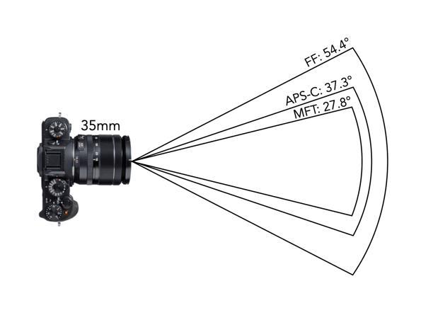
The most visible effect of crop-sensors on lenses is the angle-of-view (AOV), which is essentially where the term crop comes from – the smaller sensor’s AOV is a crop of the full frame. Take a photograph with two cameras: one with a full-frame and another with an APS-C sensor, from the same position using lens with the same focal lengths. The camera with the APS-C sensor will have a more narrowed AOV. For example a 35mm lens on a FF camera has the same focal length as a FF on an MFT or APS-C camera, however the AOV will be different on each. An example of this is shown in Fig.1 for a 35mm lens (showing horizontal AOV).
Fig.1: AOV for 35mm lenses on FF, APS-C, and MFT
Now it should be made clear that none of this affects the focal length of the lens. The focal length of a lens remains the same – regardless of the sensor on the camera. Therefore a 50mm lens in FF, APS-C or MFT will always have a focal length of 50mm. What changes is the AOV of each of the lenses, and consequently the FOV. In order to obtain the same AOV on a cropped-sensor camera, a new lens with the appropriate focal length must be chosen.
Manufacturers of crop-sensors like to use the term “equivalent focal length“. Now this is the focal length AOV as it relates to full-frame. So Olympus says that a MFT lens with a focal length of 17mm has a 34mm FF equivalency. It has an AOV of 65° (diagonal, as per the lens specs), and a horizontal AOV of 54°. Here’s how we calculate those (21.64mm is the diagonal of the MFT sensor, which is 17.3×13mm in size):
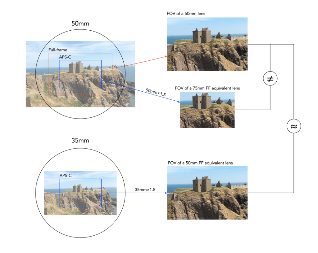
So a lens with a 17mm focal length on a camera with a 2.0× crop factor MFT sensor would give an AOV equivalent of to that of a 34mm lens. An APS-C sensor has a crop factor of ×1.5, so a 26mm lens would be required to give an AOV equivalent of the 34mm FF lens. Figure 2 depicts the differences between 50mm FF and APS-C lenses, and the similarities between a 50mm FF lens and a 35mm APS-C lens (which give approximately the same AOV/FOV).
Fig.2: Example of lens equivalencies: FF vs. APS-C (×1.5)
Interchangeability of Lenses
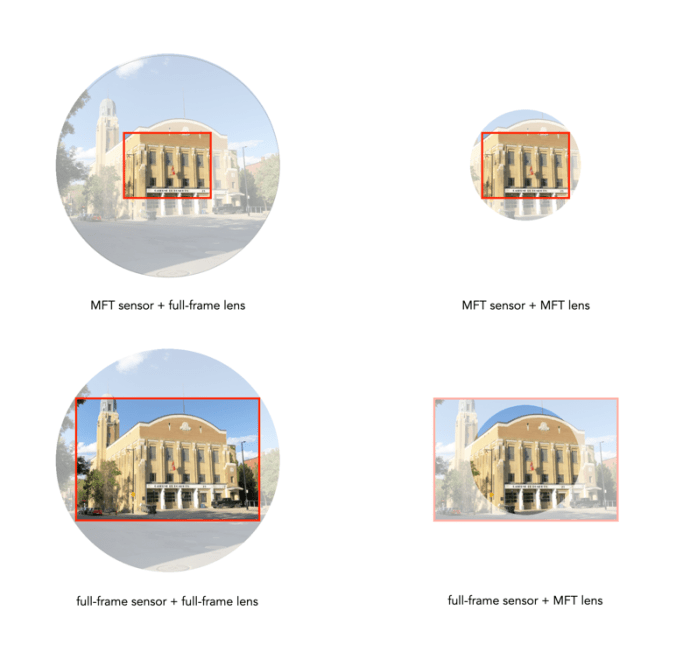
On a side note, FF lenses can be used on crop-sensor cameras because the image circle of the FF lens is larger than the crop sensor. The reverse is however not possible, as a CS lens has a smaller image circle than a FF sensor. The picture below illustrates the various combinations of FF/MFT sensor cameras, and FF/MFT lenses.
Fig.3:The effect of interchanging lenses between FF and crop sensor cameras.
Of course all this is pointless if you don’t care about comparing your crop-sensor camera to a full-frame camera.
NOTE: I tend to use horizontal AOV rather than the manufacturers more typical diagonal AOV. It makes more sense because I am generally viewing a scene in a horizontal context.
DIP is the Digital Image Processing system. Once the ADC has performed its conversion, each of the values from the photosite has been converted from a voltage to a binary number representing some value in its bit depth. So basically you have a matrix of integers representing each of the original photosites. The problem is that this is essentially a matrix of grayscale values, with each element of the matrix representing with a Red, Green of Blue pixel (basically a RAW image). If a RAW image is required, then no further processing is performed, the RAW image and its associated metadata are saved in a RAW image file format. However to obtain a colour RGB image and store it as a JPEG, further processing must be performed.
First it is necessary to perform a task called demosaicing (or demosaiking, or debayering). Demosaicing separates the red, green, and blue elements of the Bayer image into three distinct R, G, and B components. Note a colouring filtering mechanism other than Bayer may be used. The problem is that each of these layers is sparse – the green layer contains 50% green pixels, and the remainder are empty. The red and blue layers only contain 25% of red and blue pixels respectively. Values for the empty pixels are then determined using some form of interpolation algorithm. The result is an RGB image containing three layers representing red, green and blue components for each pixel in the image.
The DIP process
Next any processing related to settings in the camera are performed. For example, the Ricoh GR III has two options for noise reduction: Slow Shutter Speed NR, and High-ISO Noise Reduction. In a typical digital camera there are image processing settings such as grain effect, sharpness, noise reduction, white balance etc. (which don’t affect RAW photos). Some manufacturers also add additional effects such as art effect filters, and film simulations, which are all done within the DIP processor. Finally the RGB image image is processed to allow it to be stored as a JPEG. Some level of compression is applied, and metadata is associated with the image. The JPEG is then stored on the memory card.
The inner workings of a camera are much more complex than most people care to know about, but everyone should have a basic understanding of how digital photographs are created.
The ADC is the Analog-to-Digital Converter. After the exposure of a picture ends, the electrons captured in each photosite are converted to a voltage. The ADC takes this analog signal as input, and classifies it into a brightness level represented by a binary number. The output from the ADC is sometimes called an ADU, or Analog-to-Digital Unit, which is a dimensionless unit of measure. The darker regions of a photographed scene will correspond to a low count of electrons, and consequently a low ADU value, while brighter regions correspond to higher ADU values.
Fig. 1: The ADC process
The value output by the ADC is limited by its resolution (or bit-depth). This is defined as the smallest incremental voltage that can be recognized by the ADC. It is usually expressed as the number of bits output by the ADC. For example a full-frame sensor with a resolution of 14 bits can convert a given analog signal to one of 214 distinct values. This means it has a tonal range of 16384 values, from 0 to 16,383 (214-1). An output value is computed based on the following formula:
ADU = (AVM / SV) × 2R
where AVM is the measured analog voltage from the photosite, SV is the system voltage, and R is the resolution of the ADC in bits. For example, for an ADC with a resolution of 8 bits, if AVM=2.7, SV=5.0, and 28, then ADU=138.
Resolution (bits)
Digitizing steps
Digital values
8
256
0..255
10
1024
0.1023
12
4096
0..4095
14
16384
0..16383
16
65536
0..65535
Dynamic ranges of ADC resolution
The process is roughly illustrated in Figure 1. using a simple 3-bit, system with 23 values, 0 to 7. Note that because discrete numbers are being used to count and sample the analog signal, a stepped function is used instead of a continuous one. The deviations the stepped line makes from the linear line at each measurement is the quantizationerror. The process of converting from analog to digital is of course subject to some errors.
Now it’s starting to get more complicated. There are other things involved, like gain, which is the ratio applied while converting the analog voltage signal to bits. Then there is the least significant bit, which is the smallest change in signal that can be detected.
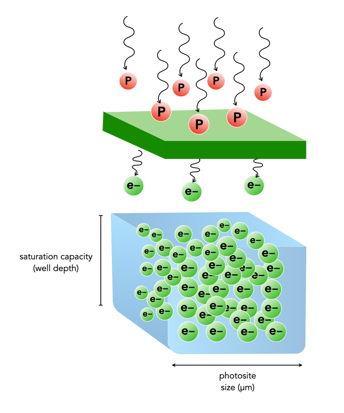
When photons (light) enter a lens of a camera, some of them will pass through all the way to the sensor, and some of those photons will pass through various layers (e.g. filters) and end up in being gathered in the photosite. Each photosite on a sensor has a capacity associated with it. This is normally known as thephotosite well capacity (sometimes called the well depth, or saturation capacity). It is a measure of the amount of light that can be recorded before the photosite becomes saturated (no long able to collect any more photons).
When photons hit the photo-receptive photosite, they are converted to electrons. The more photons that hit a photosite, the more the photosite cavity begins to fill up. After the exposure has ended, the amount of electrons in each photosite is read, and the photosite is cleared to prepare for the next frame. The number of electrons counted determines the intensity value of that pixel in the resulting image. The gathered electrons create a voltage which is an analog signal -the more photons that strike a photosite, the higher the voltage.
More light means a greater response from the photosite. At some point the photosite will not be able to register any more light because it is at capacity. Once a photosite is full, it cannot hold any more electrons, and any further incoming photons are discarded, and lost. This means the photosite has become saturated.
Fig.1: Well-depth illustrated with P representing photons, and e- representing electrons.
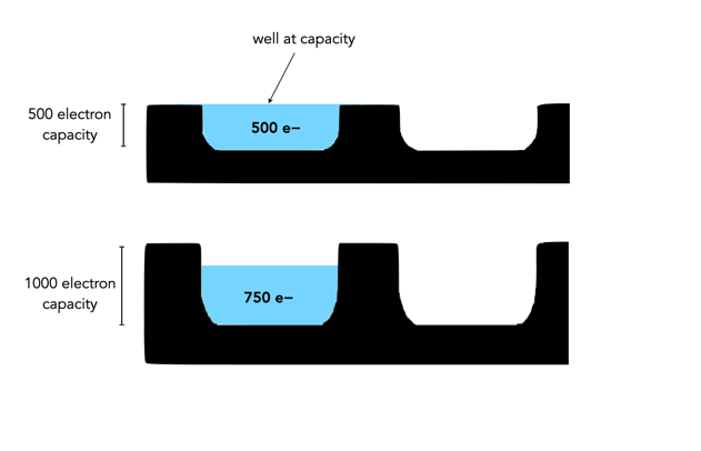
Different sensors can have photosites with different well-depths, which affects how many electrons the photosite can hold. For example consider two photosites from different sensors. One has a well-depth of 1000 electrons, and the other 500 electrons. If everything remains constant from the perspective of camera settings, noise etc., then over an exposure time the photosite with the smaller well-depth will fill to capacity sooner. If over the course of an exposure 750 photons are converted to electrons in each of the photosites, then the photosite with a well-depth of 1000 will be 75% capacity, and the photosite with a well-depth of 500 will become saturated, discarding 250 of the photons (see Figure 2).
Fig.2: Different well capacities exposed to 750 photons
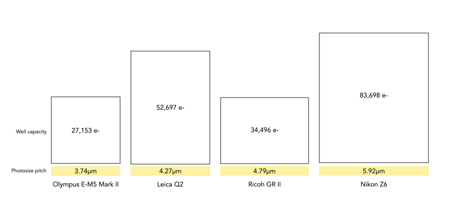
Two photosite cavities with the same well-capacities, but differing size (in μm) will also affect how quickly the cavity fills up with electrons. The larger sized photosite will fill up quicker. Figure 3 shows four differing sensors, each with a different photosite pitch, and well capacity (the area of each box abstractly represents the well capacity of the photosite in relation to the photosite pitch).
Fig.3: Examples of well capacity in various sensors
Of course the reality is that electrons do not need a physical “bin” to be stored in, the photosites are just shown in this manner to illustrate a concept. In fact the concept of well-depth is somewhat ill-termed, as it does not take into account the surface area of the photosite.