The term “crop-sensor” has become a bit nonsensical

The term “crop-sensor” doesn’t make much sense anymore, if it ever did. I understand why it evolved, because a term was needed to collectively describe smaller-than-35mm sized sensors (crop means to clip or prune, i.e. make smaller). That is, if it’s not 36×24mm in size it’s a crop-sensor. However it’s also sometimes used to describe medium-format sensors, even though they are larger than 36×24mm. In reality non-35mm sensors do provide an image which is “cropped” in terms of comparison with a full-frame sensor, but taken in isolation they are sensors unto themselves.
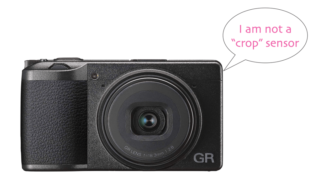
The problem lies with the notion that 36×24mm constitutes a “full-frame”, which only exists as such because manufacturers decided to continue using the concept from 35mm film SLR’s. It is true that 35mm was the core film standard for decades, but that was constrained largely by the power of 35mm film. Even half-frame cameras (18×24mm, basically APS-C size) used the same 35mm film. In the digital realm there are no constraints on a physical medium, yet we are still wholly focused on 36×24mm.

Remember, there were sub-full-frame sensors before the first true 36×24mm sensor appeared. Full-frame evolved in part because it made it easier to transition film-based lenses to digital. In all likelihood in the early days there were advantages to full-frame over its smaller brethren, however two decades later we live in a different world. “Crop” sensors should no longer be treated as sub-par players in the camera world. Yet it is this full-frame mantra that sees people ignore the benefits of smaller sensors. Yes, there are benefits to full-frame sensors, but there are also inherent drawbacks. It is the same with the concept of equivalency. We say a 33mm APS-C lens is “equivalent” to a 50mm full-frame. But why? Because some people started the trend of relating everything back to what is essentially a 35mm film format. But does there even need to be a connection between different sensors?
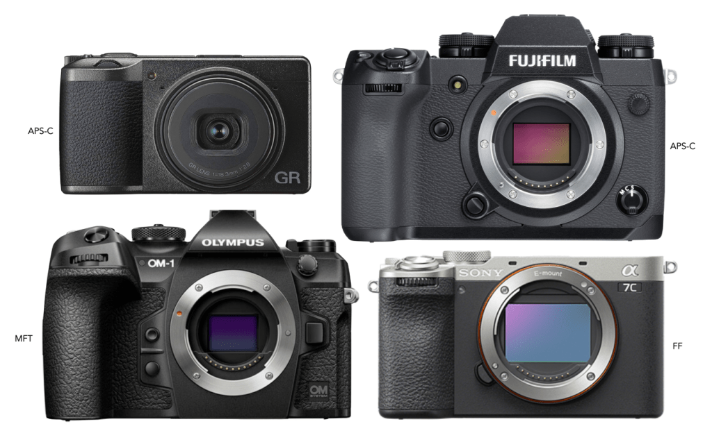
Image showing all APS-C, micro-four thirds  and full-frame cameras.
Sensor equality
What about some sensor equality?

The reason “crop” sensors have continued to evolve is because they are much cheaper to produce, and being smaller, the cameras themselves have a reduced footprint. Lenses also require less glass, making them lighter, and less expensive to manufacture. Maybe instead of using “crop-sensor”, we should just acknowledge the sensors exactly as they are: Medium, APS-C, and MFT, and change full-frame to be “35mm” format instead. So when someone talks about a 35mm sensor, they are effectively talking about a full-frame. All it takes is a little education.
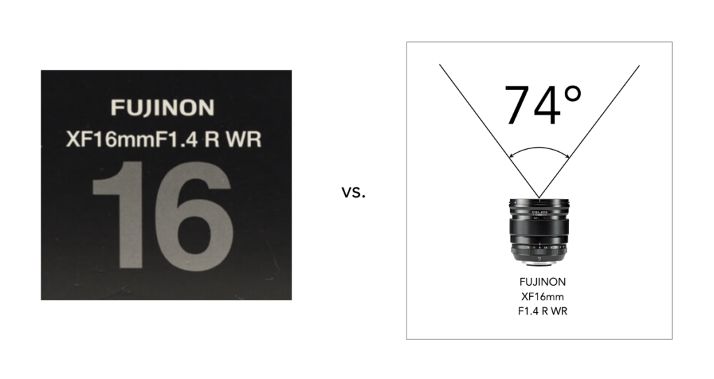
Old versus smarter advertising which puts the emphasis on the angle-of-view. In this case an Fuji APS-C lens – rather than focusing on 16mm, it focuses instead on the horizontal AOV, i.e. 74 degrees. It could also designate that the lens is a wide angle lens.

Using the term-crop sensor also does more harm than good, because it results in more terms: equivalency and crop-factor which are used in the context of focal length, AOV, and even ISO. People get easily confused and then think that a lens with a focal length of 50mm on an APS-C camera is not the same as one on a FF camera. Focal lengths don’t change, a lens that is 50mm is always 50mm. What changes is the Angle-of-View (AOV). A larger sensor gives a wider AOV, whereas a smaller sensor gives a narrower AOV. So while the 50mm lens on the FF camera has a horizontal AOV of 39.6°, the one on the APS-C camera sees only 27°.

It would be easier not to have to talk about a sensor in terms of another sensor. But even though terms like “crop-sensor” and “crop-factor” are nonsensical, in all likelihood the industry won’t change the way they perceive non-35mm sensors anytime soon. I have previously described how we could alleviate the term crop-factor as it relates to lenses, identifying lenses based on their AOV rather than purely by their focal length. This works because nearly all lenses are designed for a particular sensor, i.e. you’re not going to buy a MFT lens for an APS-C camera.
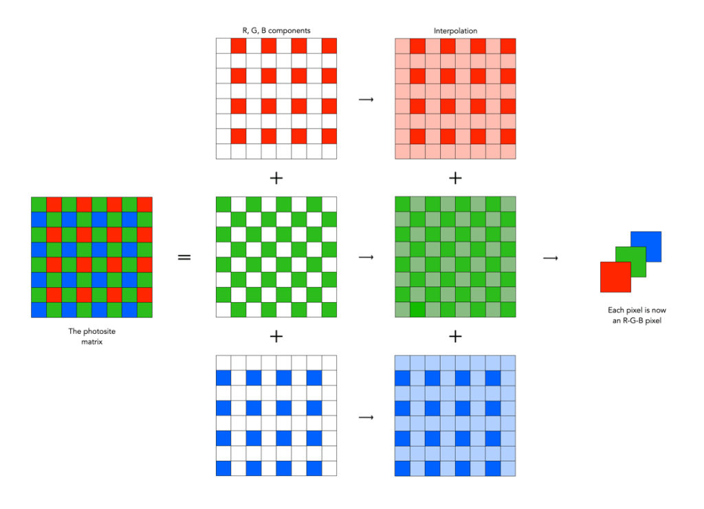
From photosites to pixels (iv) – the demosaicing process

The funny thing about the photosites on a sensor is that they are mostly designed to pick up one colour, due to the specific colour filter associated with with photosite. Therefore a normal sensor does not have photosites which contain full RGB information.

To create an image from a photosite matrix it is first necessary to perform a task called demosaicing (or demosaiking, or debayering). Demosaicing separates the red, green, and blue elements of the Bayer image into three distinct R, G, and B components. Note a colouring filtering mechanism other than Bayer may be used. The problem is that each of these layers is sparse – the green layer contains 50% green pixels, and the remainder are empty. The red and blue layers only contain 25% of red and blue pixels respectively. Values for the empty pixels are then determined using some form of interpolation algorithm. The result is an RGB image containing three layers representing red, green and blue components for each pixel in the image.

A basic demosaicing process

There are a myriad of differing interpolation algorithms, some which may be specific to certain manufacturers (and potentially proprietary). Some are quite simple, such as bilinear interpolation, while others like bicubic interpolation, spline interpolation, and Lanczos resampling are more complex. These methods produce reasonable results in homogeneous regions of an image, but can be susceptible to artifacts near edges. This leads to more sophisticated algorithms such as Adaptive Homogeneity-Directed, and Aliasing Minimization and Zipper Elimination (AMaZE).

An example of bilinear interpolation is shown in the figure below (note that no cameras actually use bilinear interpolation for demosaicing, but it offers a simple example to show what happens). For example extracting the red component from the photosite matrix leaves a lot of pixels with no red information. These empty reds are interpolated from existing red information in the following manner: where there was previously a green pixel, red is interpolated as the average of the two neighbouring red pixels; and where there was previously a blue pixel, red is interpolated as the average of the four (diagonal) neighbouring red pixels. This way the “empty” pixels in the red layer are interpolated. In the green layer every empty pixel is simply the average of the neighbouring four green pixels. The blue layer is similar to the red layer.

One of the simplest interpolation algorithms, bilinear interpolation.

❂ The only camera sensors that don’t use this principle are the Foveon-type sensors which have three separate layers of photodetectors (R,G,B). So stacked the sensor creates a full-colour pixel when processed, without the need for demosaicing. Sigma has been working on a full-frame Foveon sensor for years, but there are a number of issues still to be dealt with including colour accuracy.

Galileo’s homemade telescope

“This I did shortly afterwards, my basis being the theory of refraction. First I prepared a tube of lead , at the ends of which I fitted two glass lenses, both plane on one side while on the other side one was spherically convex. Then placing my eye near the concave lens I perceived objects satisfactorily large and near, for they appeared three times closer and nine times larger than when seen with the naked eye alone .”

− Galileo Galilei published the initial results of his telescopic observations of the heavens in Starry Messenger (Sidereus Nuncius) in 1610

Vintage camera makers – The origins of Pentacon

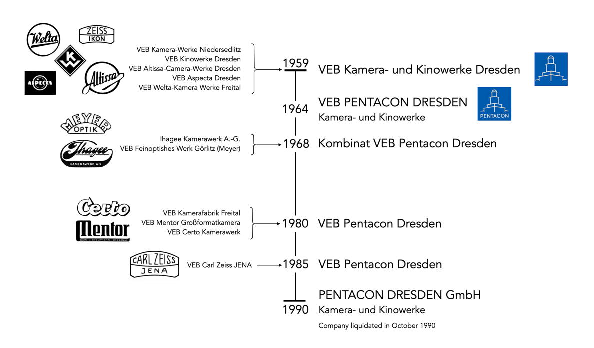
Post-WW2 there were still a lot of camera companies in Germany, and particularly in East Germany. In fact the heart of the German camera industry lay in Dresden, Jena and the surround area. Over the next decade, many of the companies were merged into a series of VEBs (Volkseigener Betrieb or Publicly Owned Enterprise) culminating with VEB Pentacon.

On January 1, 1959 a series of Dresden camera manufacturers were merged to create the large state-owned VEB Kamera und Kinowerke Dresden (KKWD). The company was a conglomerate of existing companies which produced a broad range of products and had numerous production sites. Joining them together meant production could be rationalized, yet cameras were still produced under their brands names, e.g. Contax, Welta, Altissa, Reflekta, Belfoca.

  • VEB Kinowerke Dresden − Formerly VEB Zeiss Ikon
  • VEB Kamera-Werke Niedersedlitz − This is where the Praktiflex, precursor of the Praktica, was invented; it included VEB Belca-Werk absorbed in 1957.
  • VEB Welta-Kamera Werke Freital − This included the VEB Reflekta-Kamerawerk Tharandt and Welta-Kamera-Werk Freital (Reflekta II, Weltaflex und Penti).
  • VEB Altissa Kamerawerke Dresden − Formerly Altissa-Camera-Werk Berthold Altmann, (including Altissa, Altiflex and Altix cameras).
  • VEB Aspecta Dresden − Formerly Filmosto-Projektoren Johannes (including projectors, enlargers, lenses).

In 1964 the company was renamed to VEB Pentacon Dresden Kamera-und Kinowerke. This was intended to provide a catchy name for the company (not forgetting that a lot of its products were intended for Western markets). Pentacon was already being used as the export name for the mirror Contax D, and was derived from PENTAprisma and CONtax. Pentacon used the stylized silhouette of the Ernemann Tower (on the old Ernemann camera factory site, which belonged to the former Zeiss Ikon) as its corporate logo. The company continued to produce good SLRs: Praktica V (1964), Praktica Nova with return mirror (1964), Praktica Nova B with uncoupled light meter (1965), Praktica Mat for the first time with TTL interior light metering (1965). In 1966 the 6×6 format Pentacon Six appeared, with the Praktica PL Nova I in 1967.

The evolution of Pentacon

On January 2, 1968, the VEB was restructured, and more companies were added into the fold, including Ihagee Kamerawerk (which had remained independent until this point), and VEB Feinoptisches Werk Görlitz. The name became Kombinat VEB Pentacon Dresden.

  • Ihagee Kamerawerk AG i.V. − Produced Exakta and Exa cameras.
  • VEB Feinoptisches Werk Görlitz − Formerly Meyer-Optik Görlitz

The continuous expansion and bundling of technical expertise and concentration of the production capacities of the Pentacon, led to the incorporation of three more companies in 1980.

  • VEB Kameratechnik Freital − Formerly Freitaler camera industry Beier & Co., including Beirette cameras.
  • VEB Mentor Großformatkamera − large format cameras
  • VEB Certo Kamerawerk Dresden − folding cameras

On January 1, 1985, the VEB Pentacon, which by now had absorbed most of the East German camera industry was formally incorporated into Kombinat VEB Carl Zeiss Jena. This move amalgamated nearly the entire East German photography industry under the Zeiss umbrella. There were scarce few years between this and the reunification of Germany. After reunification, VEB Carl Zeiss Jena was reabsorbed into the Stiftung and was completely restructured. VEB Pentacon was renamed PENTACON DRESDEN GmbH, in July 1990, but by October it was being liquidated.

What is a mirrorless camera?

It is a camera without a mirror of course!
Next you’ll ask why a camera would ever need a mirror.

Over the last few years we have seen an increased use of the term “mirrorless” to describe cameras. But what does that mean? Well, 35mm SLR (Single Lens Reflex) film cameras all contained a reflex mirror. The mirror basically redirects the light (i.e. view) coming through the lens to the film by means of a pentaprism, to the optical viewfinder (OVF) – which is then viewed by the photographer. Without it, the photographer would have to view the scene by means of an offset window (like in a rangefinder camera, which were technically mirrorless). This basically means that the photographer sees what the lens sees. When the photographer presses the shutter-release button, the mirror swings out of the way, temporarily blocking the light from passing through the viewfinder, and instead allowing the light to pass through the opened shutter onto the film. This is depicted visually in Figure 1.

Fig.1: A cross-section of a 35mm SLR camera showing the mirror and optical viewfinder (OVF)

When DSLR (Digital Single Lens Reflex) cameras appeared they used similar technology. The problem is that this mirror, together with the digital electronics, meant that the cameras became larger than traditional film SLRs. The concept of mirrorless cameras appeared in 2008, with the introduction of the Micro-Four-Thirds system. The first mirrorless interchangeable lens camera was the Panasonic Lumix DMC-G1. It replaced the optical path of the OVF with an electronic viewfinder (EVF), making it possible to remove the mirror completely, hence reducing the size of cameras. The EVF shows the image that the sensor outputs, displaying the output on a small LCD or OLED screen.

Fig.2: DSLR versus a mirrorless camera. In the DLSR the light path to the OVF by means of the mirror is shown in blue. When the shutter-release button is pressed, the mirror retracts (pink mirror), and the light is allowed to pass through to the sensor (pink path).

As a result of nixing the mirror, mirrorless cameras are typically have fewer moving parts, and are slimmer than DSLRs, shortening the distance between the lens and the sensor. The loss of the mirror also means that it is easier to adapt vintage lenses for use on digital cameras. Some people still prefer using an OVF, because it is optical, and does not require as much battery-life as an EVF.

These days the only cameras still containing mirrors are usually full-frame DSLRs, and they are slowly disappearing, replaced by mirrorless cameras. Basically all recent crop-sensor cameras are mirrorless. DSLR sales continue to decline. Looking only at interchangeable lens cameras (ILC), according to CIPA, mirrorless cameras in 2022 made up 68.7% of all ILD units (4.07M versus 1.85M), and 85.8% of shipped value (out of 5.927 million units shipped).

How natural light and meaningful darkness tell a story

Have you ever been somewhere, and want to take a photograph, and there just isn’t much natural light, or perhaps the light is only coming from a single source, such as a window? Are you tempted to use a flash? Well don’t even think about it, because doing so takes away from the story of what you are photographing. Usually this sort of scenario manifests itself inside historical buildings where there just isn’t much natural light, and in context, no artificial light. Think anything before electric lighting – houses, castles, outbuildings, etc. Photography in historical buildings can be burdened by a lack of light – but that’s how they were when inhabited.

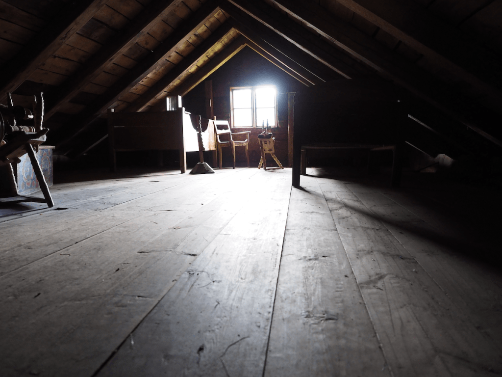
I photograph mostly using natural light. I don’t like using a flash, because ultimately there are certain qualities of natural light that enhance the colours and aesthetics of an object or scene. I find flash light too harsh, even when used with diffusers. But that’s just me. Below is an image from the attic space of a building at the Voss Folkemuseum in Norway. The room contained some beds, and storage chests, so obviously it was used as a bedroom. The light streaming through the window is enough to bathe the room with enough light to show its use (typically windows would only have been installed where the light would be most concentrated, in this case south-facing). Notice the spinning wheel next to the window where the light is most concentrated?

An attic space in a building at the Voss Folkemuseum in Voss, Norway.

A lack of light often tells a story. It shows you what the space really was like for those who inhabited it long ago. Before the advent of electricity, most buildings relied on natural light during the day, and perhaps candle-light at night. Windows were small because glass was inherently expensive, and the more glass one had, the more heat that was lost in winter. If you were documenting a scene in a more archival manner, you might naturally flood the scene with artificial light of a sort, but historical photography should not be harshly lit.

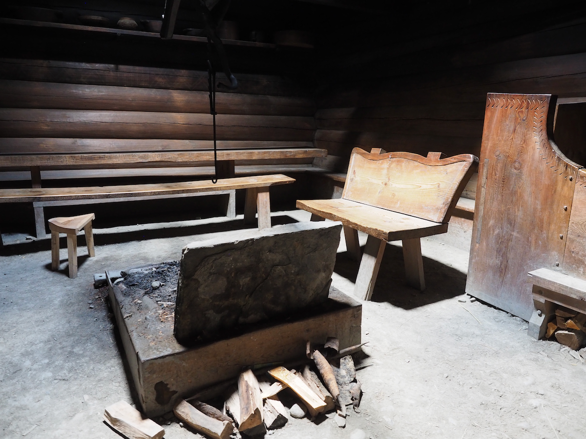
Many historic buildings were built at a time of very little beyond natural light and candles. The light today is that very same light, and to bath it with artificial light would be unnatural. These nooks and crannies were never meant to be bathed in complete light. Consider the images below, taken at different folke-museums in Norway. The images are of cooking fires inside historic buildings, which had no openings except in the roof. The one from the Norsk Folkemuseum is Saga-Stau, a replica of an open-hearth house from about 3000 years ago.

The inside of an open-hearth house at the Norsk Folkemuseum
Eldhus (house with fireplace and bakehouse) at Voss Folkemuseum

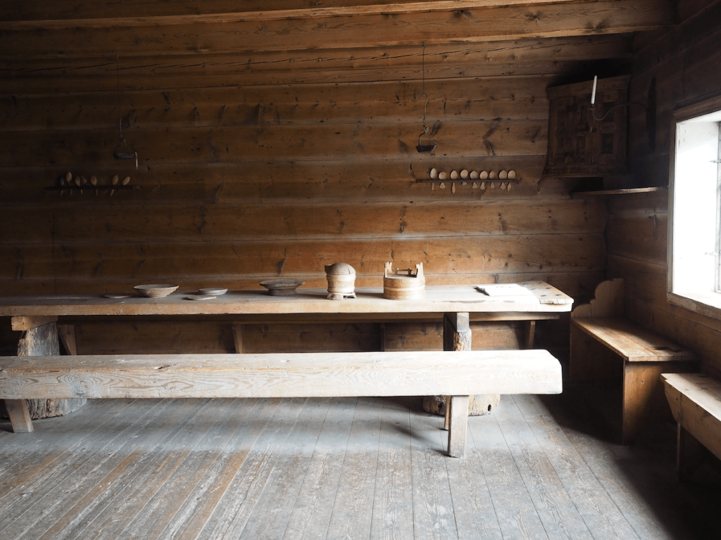
On a bright sunny day, dark spaces are bathed in whatever available light is able to seep through every opening. In a dark space this light can often appear harsh, blinding window openings to the point where there is little cognition of the scene beyond the window. Yet it also tends to produce shards of light puncturing into a space. On clouded days, the light can be more muted. In the image below of the living space, the light coming through the window is harsh enough to produce highlight clipping of both the window frame and part of the table. However the light adds a sense of Norwegian Hygge to the entire scene. To light this scene with a flash would simply reduce the scene to a series of artifacts, rather than a slice of history.

An indoor scene at the Voss Folkemuseum.

Upgrading camera sensors – the megapixel phenomena

So if you are planning to purchase a new camera with “upgraded megapixels”, what makes the most sense? In many cases, people will tend to continue using the same brand or sensor. This makes sense from the perspective of existing equipment such as lenses, but sometimes an increase in resolution requires moving to a new sensor. There are of course many things to consider, but the primary ones when it comes to the images produced by a sensor are: aggregate MP and linear dimensions (we will consider image pixels rather than sensor photosites). Aggregate MP are the total number of pixels in an image, whereas linear dimensions relate to the width and height of an image. Doubling the number of pixels in an image does not double an images linear dimensions. Basically doubling the megapixels will double the aggregate megapixels in an image. To double the linear dimensions of an image, the megapixels need to be quadrupled. So 24MP needs to ramp up to 96MP in order to double the linear dimensions.

Table 1 shows some sample multiplication factors for aggregate and linear dimensions when upgrading megapixels, ignoring sensor size. The image sizes offer a sense of what is what is offered, with the standard MP sizes offered by various manufacturers shown in Table 2.

16MP24MP30MP40MP48MP60MP
16MP1.5 (1.2)1.9 (1.4)2.5 (1.6)3.0 (1.7)3.75 (1.9)
24MP1.25 (1.1)1.7 (1.3)2.0 (1.4)2.5 (1.6)
30MP1.3 (1.2)1.6 (1.3)2.0 (1.4)
40MP1.2 (1.1)1.5 (1.2)
48MP1.25 (1.1)
Table 1: Changes in aggregate megapixels, and (linear dimensions) shown as multiplication factors.

Same sensor, more pixels

First consider a different aggregate of megapixels on the same size sensor – the example compares two Fuji cameras, both of which use an APS-C sensor (23.6×15.8mm).

Fuji X-H2 − 40MP, 7728×5152
Fuji X-H2S − 26MP, 6240×4160

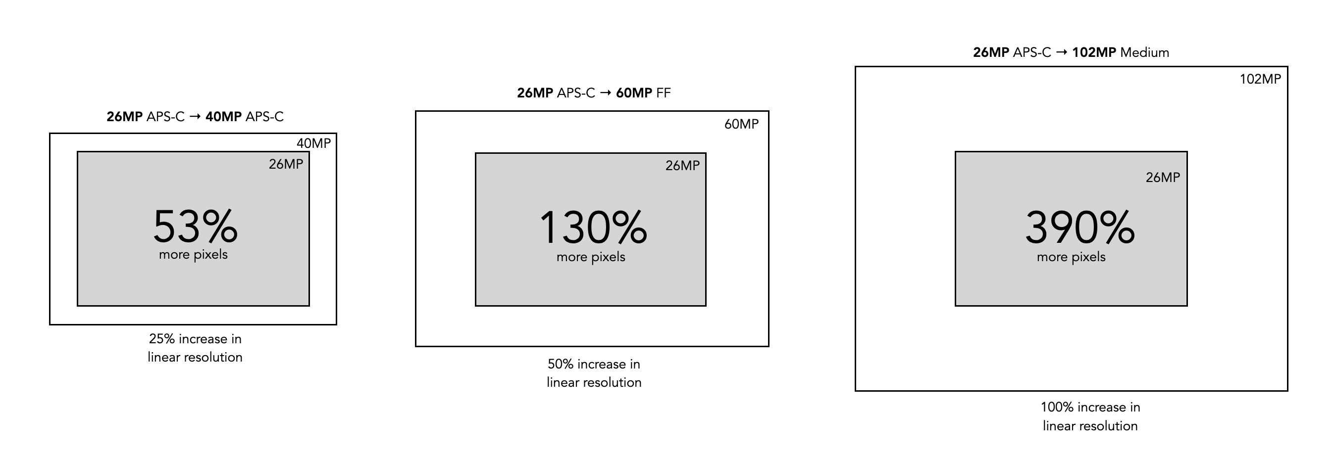
So there are 1.53 times more pixels in the 40MP sensor, however from the perspective of linear resolution (comparing dimensions), there is only a 1.24 times differential. This means that horizontally (and vertically) there are only one-quarter more pixels in the 40MP versus the 26MP. But because they are on the same size sensor, the only thing that really changes is the size of the photosites (known as the pitch). Cramming more photosites on a sensor means that the photosites get smaller. In this case the pitch reduces from 3.78µm (microns) in the X-H2S to 3.05µm in the X-H2. Not an incredible difference, but one that may affect things such as low-light performance (if you care about these sort of things).

A visualization of differing sensor size changes

Larger sensor, same pixels

Then there is the issue of upgrading to a larger sensor. If we were to upgrade from an APS-C sensor to an FF sensor, then we typically get more photosites on the sensor. But not always. For example consider the following upgrade from a Fuji X-H2 to a Leica M10-R:

FF: Leica M10-R (41MP, 7864×5200)
APS-C: Fuji X-H2 (40MP, 7728×5152)

So there are very few differences from the perspective of either image resolution, or linear resolution (dimensions). The big difference here is the photosite pitch. The Leica has a pitch of 4.59µm, versus the 3.05µm of the Fuji. From the perspective of photosite area, this means that 21µm² versus 9.3µm², or 2.25 times the light-gathering space on the full-frame sensor. How much difference this makes from the perspective of the end-picture is uncertain due to the multiplicities of factors involved, and computational post-processing each camera provides. But it is something to consider.

Larger sensor, more pixels

Finally there is upgrading to more pixels on a larger sensor. If we were to upgrade from an APS-C sensor (Fuji X-H2S) to a FF sensor (Sony a7R V) with more pixels:

FF: Sony a7R V (61MP, 9504×6336)
APS-C: Fuji X-H2S (26MP, 6240×4160)

Like the first example, there are 2.3 times more pixels in the 61 MP sensor, however from the perspective of linear resolution, there is only a 1.52 times differential. The challenge here can be that the photosite pitch can actually remain the same. The pitch on the Fuji sensor is 3.78µm, versus the 3.73µm of the Sony.

brandMFTAPS-CFull-frameMedium
Canon24, 3324, 45
Fuji16, 24, 26, 4051, 102
Leica1716, 2424, 41, 47, 60
Nikon21, 2424, 25, 46
OM/Olympus16, 20
Panasonic20, 2524, 47
Sony24, 2633, 42, 50, 60, 61
Table 2: General megapixel sizes for the core brands

Upgrading cameras is not a trivial thing, but one of the main reasons people do so is more megapixels. Of all the brands listed above, only one, Fuji, has taken the next step, and introduced a medium format camera (apart from the medium format camera manufacturers, e.g. Hasselblad), allowing for increased sensor size and increased pixels, but not at the expense of photosite size. The Fujifilm GFX 100S has a medium format sensor, 44×33mm in size, providing 102MP with 3.76µm. This means it provides approximately double the dimensional pixels as a Fuji 24MP APS-C camera (and yes it costs almost three times as much, but there’s no such thing as a free lunch).

At the end of the day, you have to justify why more pixels are needed to yourself. They are only part of the equation in the acquisition of good images, but small upgrades like 24MP to 40MP may not actually provide much of a payback.

Vintage lens makers – Piesker (Germany)

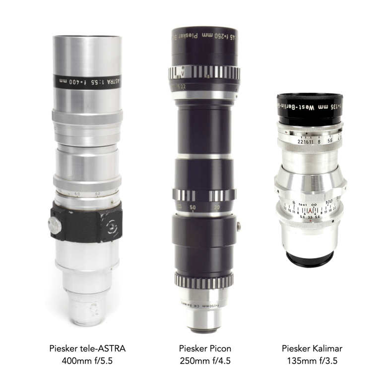
Paul Piesker & Co. was founded in 1936 as a Berlin manufacturer of lenses and lens accessories for reflex cameras (in West Germany). After WW2 the company focused on lenses with long focal lengths for the Exakta and cameras with M42 mounts. Like its competitors, Astro-Berlin, and Tewe, Piesker lenses don’t seem to very common, at least not in Europe. Most of the lenses produced seem to have been for the US market, where they appeared in ads in Popular Photography in the mid 1950s. The lenses can also be found under the “Kalimar” trademark, and also rebranded for Sterling Howard, under the trademark “Astra”, and “Voss” (in addition to other brands: Picon, Votar, Telegon). Production at Piesker was discontinued in 1964.

Are (camera-based) RGB histograms useful?

When taking an image on a digital camera, we are often provided with one or two histograms – the luminance histogram, and the RGB histogram. The latter is often depicted in various forms: as a single histogram showing all three channels of the RGB image, or three separate histograms, one for each of R, G, and B. So how useful is the RGB histogram on a camera? In the context of improving image quality RGB histograms provide very little in the way of value. Some people might disagree, but fundamentally adjusting a picture based on the individual colour channels on a camera, is not realistic (and usually it is because they don’t have a real understanding about how colour spaces work).

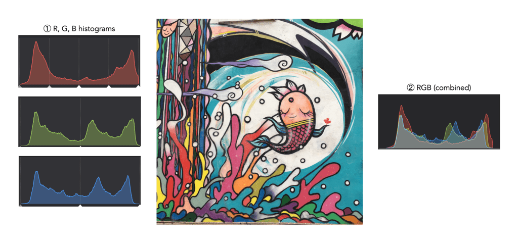
Consider the image example shown in Figure 1. This 3024×3024 pixel image has 9,144,576 pixels. On the left are the three individual RGB histograms, while on the right is the integral RGB histogram with the R, G, B, histograms overlapped. As I have mentioned before, there is very little information which can be gleaned by looking at the these two-dimensional RGB histograms – they do not really indicate how much red (R), green (G), or blue (B) there is in an image, because these three components can only be used together to produce information that is useful. This is because RGB is a coupled colour space where luminance and chrominance are coupled together. The combined RGB histogram is especially poor from an interpretation perspective, because it just muddles the information.

Fig.1: The types of RGB histograms found in-camera.

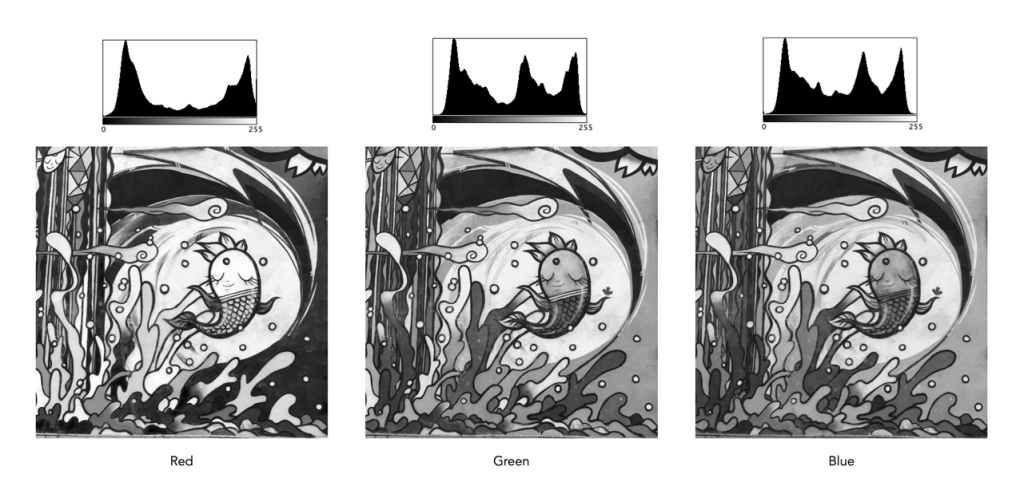
But to understand it better, we need to look at what information is contained in a colour image. An RGB colour image can be conceptualized as being composed of three layers: a red layer, a green layer, and a blue layer. Figure 2 shows the three layers of the image in Figure 1. Each layer represents the values associated with red, green, and blue. Each pixel in a colour image is therefore a set of triplet values: a red, a green, and a blue, or (R,G,B), which together form a colour. Each of the R, G, and B components is essentially an 8-bit (grayscale) image, then can be viewed in the form of a histogram (also shown in Figure 2 and nearly always falsely coloured with the appropriate red, green or blue colour).

Fig.2: The R, G, B components of RGB.

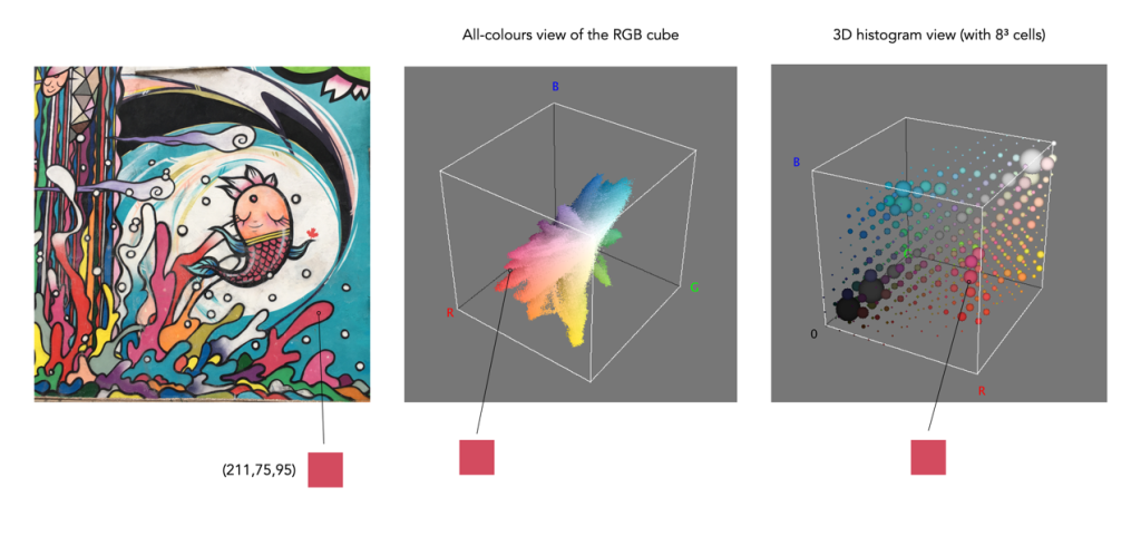
To understand a colour image further, we have to look at the RGB colour model, the method used in most image formats, e.g. JPEG. The RGB model can be visualized in the shape of a cube, formed using the R, G, and B data. Each pixel in an image has an (R, G, B) value which provides a coordinate in the 3D space of the cube (which contains 2563, or 16,777,216 colours). Figure 3 shows two different ways of viewing image colour in 3D. The first is an all-colours view of the colours. This basically just indicates all the colours contained in the image without frequency information. This gives an overall indication on how colours are distributed. In the case of the example image, there are 526,613 distinct colours. The second cube is a frequency-based 3D histogram, grouping like data together in “bins”, in this example the 3D histogram has 83 or 512 bins (which is honestly easier to digest than 16 million-odd bins). Within the image there is shown one pixel with the RGB value (211,75,95), and its location in the 3D histograms.

Fig.3: How to really view the colours in RGB

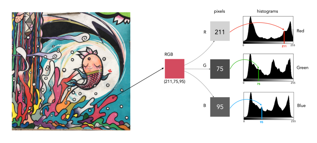
In either case, visually you can see the distribution of colours. The same can not be said of many of the 2D representations. Let’s look at how the colour information pans out in 2D form. The example image pixel in Figure 3 at location (2540,2228) has the RGB value (211,75,95). If we look at this pixel in the context of the red, green, and blue histograms it exists in different bins (Figure 4). There is no way that these 2D histograms provide anything in the way of context on the distribution of colours. All they do is show the distribution of red, green, and blue values, from 0 to 255. What the red histogram tells us is that at value 211 there are 49972 colour pixels in the image whose first value of the triplet (R) is 211. It may also tell us that the contribution of red in pixels appears to be constrained to the upper and lower bounds of the histogram (as shown by the two peaks). There is only one pure value of red, (255,0,0). Change the value from (211,75,95) to (211,75,195) and we get a purple colour.

Fig.4: A single RGB pixel shown in the context of the separate histograms.

The information in the three histograms is essentially decoupled, and does not provide a cohesive interpretation of colours in the image, for that you need a 3D image of sorts. Modifying one or more of the individual histograms will just lead to a colour shift in the image, which is fine if that is the what is to be achieved. Should you view the colour histograms on a camera viewscreen? I honestly wouldn’t bother. They are more useful in an image manipulation app, but not in the confines of a small screen – stick to the luminance histogram.

What is a micron?

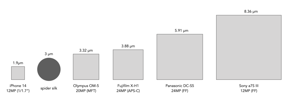
The nitty-gritty of digital camera sensors takes things down to the micron. For example the width of photosites on a sensor is measured in microns, more commonly represented using the unit µm, e.g. 3.71µm. But what is a micron?

Various sensor photosite sizes compared to spider silk (size is exaggerated of course).

Basically a micron is a micrometre, a metric unit of measure for length equal to 0.001 mm (or 1/1000mm). I mean it’s small, like really small. To put it also into perspective table salt has a particle size of 120µm. Human hair has an average diameter of 70µm, milled flour can be anywhere in the range 25-200µm, and spider silk is a measly 3µm.

To put it another way, for a photosite that is 3.88µm in size, we could fit 257 of them in just 1mm of space.