This is the first post in an ongoing series that looks at the intensity histograms of various images, and what they help tell us about the image. The idea behind it is to try and dispel the myths behind the “ideal” histogram phenomena, as well as helping to learn to read a histogram. The hope is to provide a series of posts (each containing three images and their histograms) based on histogram concepts such as shape, of clipping etc. Histograms are interpreted in tandem with the image.
Histogram 1: Ideal with a hint of clipping
The first image is the poster-boy for “ideal” histograms (almost). A simple image of a track through a forest in Scotland, it has a beautiful bell-shaped (unimodal) curve, almost entiorely in the midtones. A small amount of pixels, less than 1%, form a highlight clipping issue in the histogram, a result of the blown-out, overcast sky. Otherwise it is a well-formed image with good contrast and colour.
Histogram 2: The witches hat
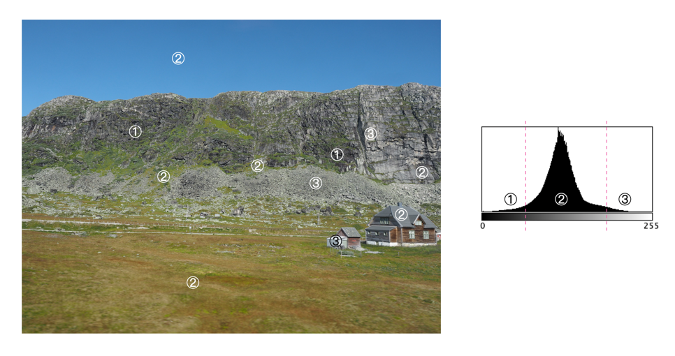
This is a picture taken along the route of the Bergen-Line train in Norway. A symmetric, unimodal histogram, taking on a classic “witches hat” shape. The tail curving towards 0 (①) deals with the darker components of the upper rock-face, and the house. The tail curving towards 255 (③) deals with the lighter components of the lower rock face, and the house. The majority of midtone pixels form the sky, grassland, and rock face.
Olympus E-M5MArkII (16MP): 12mm; f/6.3; 1/400
Histogram 3: An odd peak
This is a photograph of the statue of Leif Eriksson which is in front of Reykjavik’s Hallgrímskirkja. It provides for a truly odd histogram – basically the (majority of) pixels form a unimodal histogram, ③ , which represents the sky surrounding the statue. The tiny hillocks to either side (①,②) form the sculpture itself – the left forming the shadows, and the right forming the bright regions. However overall, this is a well formed image, even though it may appear as if the sculpture is low contrast.
One of the most important characteristics of a histogram is its shape. A histogram’s shape offers a good indicator of an image’s ability to tolerate manipulation. A histogram shape can help elucidate the overall contrast in the image. For example a broad histogram usually reflects a scene with significant contrast, whereas a narrow histogram reflects less contrast, with an image which may appear dull or flat. As mentioned previously, some people believe an “ideal” histogram is one having a shape like a hill, mountain, or bell. The reality is that there are as many shapes as there are images. Remember, a histogram represents the pixels in an image, not their position. This means that it is possible to have a number of images that look very different, but have similar histograms.
The shape of a histogram is usually described in terms of simple shape features. These shape features are often described using geographical terms (because a histogram often reminds people of the profile view of a geographical feature): e.g. “hillock” or “mound”, which is a shallow, low feature, “hill” or “hump”, which is a feature rising higher than the surrounding areas, a “peak”, which is a feature with a distinctly top, a “valley”, which is a low area between two peaks, or a “plateau” which is a level region between other features. Features can either be distinct, i.e. recognizably different, or indistinct, i.e. not clearly defined, often blended with other features. These terms are often used when describing the shape of a particular histogram in detail.
Fig.1: A sample of feature shapes in a histogram
From the perspective of simplicity, however histogram shapes can be broadly classified into three basic categories (examples are shown in Fig.2):
Unimodal – A histogram where there is one distinct feature, typically a hump or peak, i.e. a good amount of an image’s pixels are associated with the feature. The feature can exist anywhere in the histogram. A good example of a unimodal histogram is the classic “bell-shaped” curve with a prominent ‘mound’ in the center and similar tapering to the left and right (e.g. Fig.2: ①).
Bimodal – A histogram where there are two distinct features. Bimodal features can exist as a number of varied shapes, for example the features could be very close, or at opposite ends of the histogram.
Multipeak – A histogram with many prominent features, sometimes referred to as multimodal. These histograms tend to differ vastly in their appearance. The peaks in a multipeak histogram can themselves be composed of unimodal or bimodal features.
These categories can can be used in combination with some qualifiers (numeric examples refer to Figure 2). For example a symmetric histogram, is a histogram where each half is the same. Conversely an asymmetric histogram is one which is not symmetric, typically skewed to one side. One can therefore have a unimodal, asymmetric histogram, e.g. ⑥ which shows a classic “J” shape. Bimodal histograms can also be asymmetric (⑪) or symmetric (⑬).
Fig.2: Core categories of histograms: unimodal, bimodal, multi-peak and other.
Histograms can also be qualified as being indistinct, meaning that it is hard to categorize it as any one shape. In ㉓ there is a peak to the right end of the histogram, however the major of the pixels are distributed in the uniform plateau to the right. Sometimes histogram shapes can also be quite uniform, with no distinct groups of pixels, such as in example ㉒ (in reality though these images are quite rare). It it also possible that the histogram exhibits quite a random pattern, which might only indicate quite a complex scene.
But a histogram’s shape is just its shape. To interpet a histogram requires understanding the shape in context to the contents of the scene within the image. For example, one cannot determine an image is too dark from a left-skewed unimodal histogram without knowledge of what the scene entails. Figure 3 shows some sample colour images and their corresponding histograms, illustrating the variation existing in histograms.
Fig.3: Various colour images and their corresponding intensity histograms