Choosing an APS-C camera: 26MP or 40MP?

April 21, 2025 / spqr / Leave a comment

The most obvious choice when it comes to APS-C cameras is usually the number of megapixels. Not that there is really that much to choose from. Usually it is a case of 24/26MP or 40MP. Does the jump to 40MP really make all that much difference? Well, yes and no. To illustrate this we will compare two Fujifilm cameras: (i) the 26MP X-M5 with 6240×4160 photosites, and (ii) the 40MP X-T50 with 7728×5152 photosites.

Firstly, an increase in megapixels just means that more photosites have been crammed onto the sensor, and as a result they have been reduced in size (sensor photosites have dimensions, whereas image pixels are dimensionless). The size of the photosites in the X-M5 is 3.76µm, versus 3.03µm for the X-T50. This is a 35% reduction in the area of a photosite on the X-T50 relative to the X-M5, which might or might not be important (it is hard to truly compare photosites given the underlying technologies and number of variables involved).

*Fig.1: Comparing various physical aspects of the 26MP and 40MP APS-C sensors (based on the example Fuji cameras).*

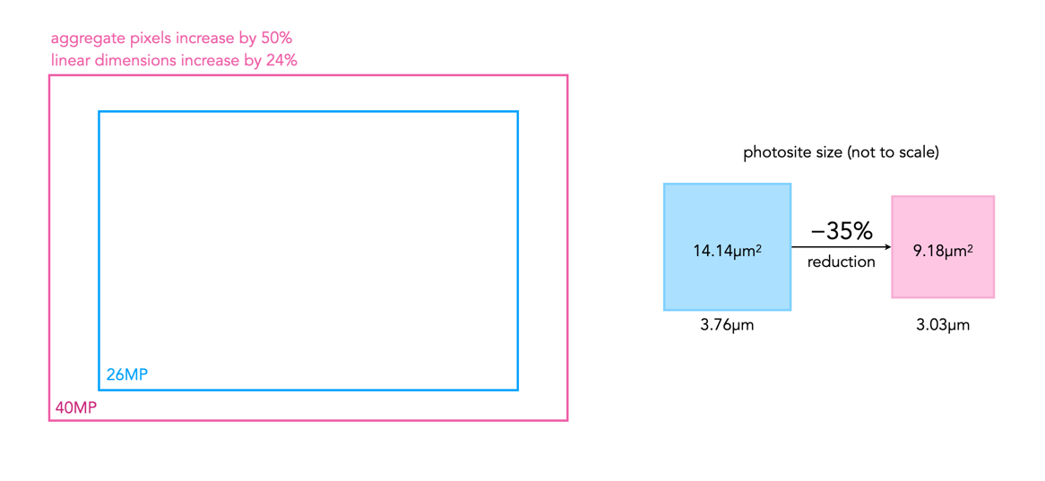
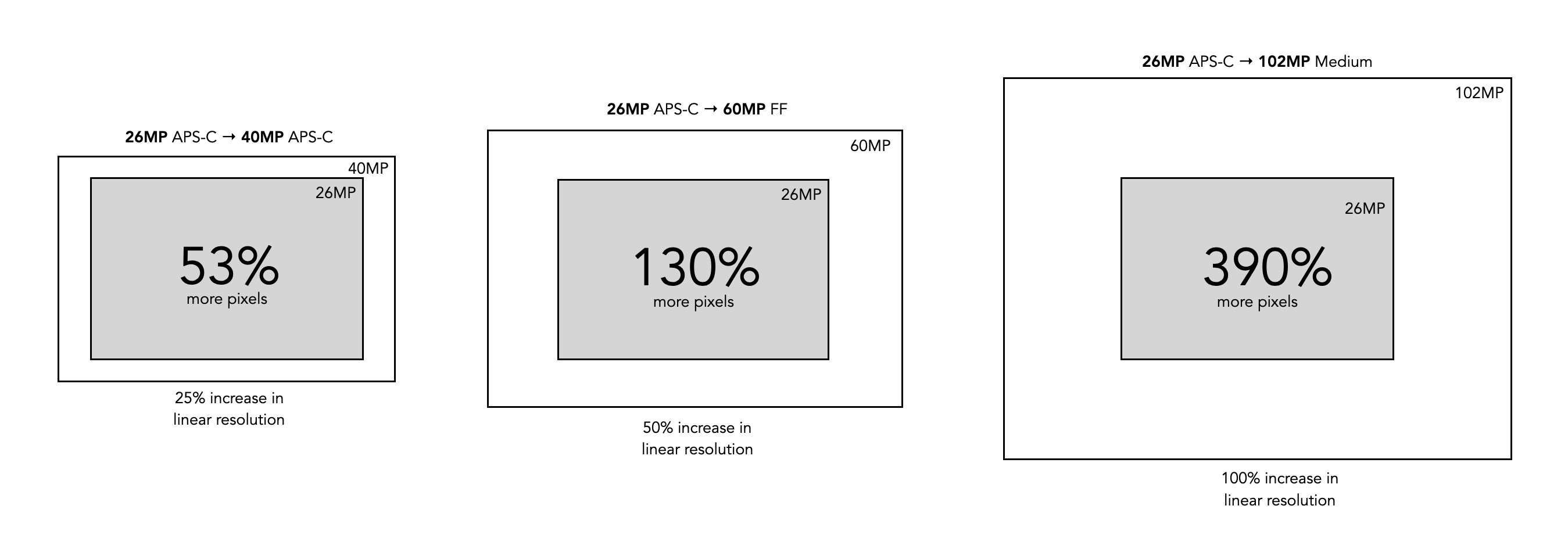
Secondly, from an image perspective, a 40MP sensor will produce an image with more aggregate pixels in it than a 26MP image, 1.5 times more in fact. But aggregate pixels only relate to the total amount of pixels in the resulting image. The other thing to consider is the linear dimensions of an image, which relates to its width and height. Increasing the amount of pixels in an image by 50% does not increase the linear dimensions by 50%. For example doubling the photosites on a sensor will double the aggregate pixels in an image. However to double the linear dimensions of an image, the number of photosites on the sensor need to be quadrupled. So 26MP needs to ramp up to 104MP in order to double the linear dimensions. So the X-T50 will produce an image with 39,814,656 pixels in it, versus 25,958,400 pixels for the X-M5. This relates to 1.53 times as many aggregate pixels. However the linear dimensions only increase 1.24 times, as illustrated in Fig.1.

So is the 40MP camera better than the 26MP camera? It does produce images with slightly more resolution, because there are more photosites on the sensor. But the linear dimensions may not warrant the extra cost in going from 26MP to 40MP (US$800 versus US$1400 for the sample Fuji cameras, body only). The 40MP sensor does allow for a better ability to crop, and marginally more detail. It also allows for the ability to print larger posters. Conversely the images are larger, and take more computational resources to process.

At the end of the day, it’s not about how many image megapixels a camera can produce, it’s more about clarity, composition, and of course the subject matter. Higher megapixels might be important for professional photographers or for people who focus on landscapes, but as amateurs, most of us should be more concerned with capturing the moment rather than getting going down the rabbit hole of pixel count.

Further reading:

From photosites to pixels (iv) – the demosaicing process

September 6, 2023 / spqr / Leave a comment

The funny thing about the photosites on a sensor is that they are mostly designed to pick up one colour, due to the specific colour filter associated with with photosite. Therefore a normal sensor does not have photosites which contain full RGB information.

To create an image from a photosite matrix it is first necessary to perform a task called demosaicing (or demosaiking, or debayering). Demosaicing separates the red, green, and blue elements of the Bayer image into three distinct R, G, and B components. Note a colouring filtering mechanism other than Bayer may be used. The problem is that each of these layers is sparse – the green layer contains 50% green pixels, and the remainder are empty. The red and blue layers only contain 25% of red and blue pixels respectively. Values for the empty pixels are then determined using some form of interpolation algorithm. The result is an RGB image containing three layers representing red, green and blue components for each pixel in the image.

There are a myriad of differing interpolation algorithms, some which may be specific to certain manufacturers (and potentially proprietary). Some are quite simple, such as bilinear interpolation, while others like bicubic interpolation, spline interpolation, and Lanczos resampling are more complex. These methods produce reasonable results in homogeneous regions of an image, but can be susceptible to artifacts near edges. This leads to more sophisticated algorithms such as Adaptive Homogeneity-Directed, and Aliasing Minimization and Zipper Elimination (AMaZE).

An example of bilinear interpolation is shown in the figure below (note that no cameras actually use bilinear interpolation for demosaicing, but it offers a simple example to show what happens). For example extracting the red component from the photosite matrix leaves a lot of pixels with no red information. These empty reds are interpolated from existing red information in the following manner: where there was previously a green pixel, red is interpolated as the average of the two neighbouring red pixels; and where there was previously a blue pixel, red is interpolated as the average of the four (diagonal) neighbouring red pixels. This way the “empty” pixels in the red layer are interpolated. In the green layer every empty pixel is simply the average of the neighbouring four green pixels. The blue layer is similar to the red layer.

*One of the simplest interpolation algorithms, bilinear interpolation.*

❂ The only camera sensors that don’t use this principle are the Foveon-type sensors which have three separate layers of photodetectors (R,G,B). So stacked the sensor creates a full-colour pixel when processed, without the need for demosaicing. Sigma has been working on a full-frame Foveon sensor for years, but there are a number of issues still to be dealt with including colour accuracy.

Upgrading camera sensors – the megapixel phenomena

August 14, 2023 / spqr / 2 Comments

So if you are planning to purchase a new camera with “upgraded megapixels”, what makes the most sense? In many cases, people will tend to continue using the same brand or sensor. This makes sense from the perspective of existing equipment such as lenses, but sometimes an increase in resolution requires moving to a new sensor. There are of course many things to consider, but the primary ones when it comes to the images produced by a sensor are: aggregate MP and linear dimensions (we will consider image pixels rather than sensor photosites). Aggregate MP are the total number of pixels in an image, whereas linear dimensions relate to the width and height of an image. Doubling the number of pixels in an image does not double an images linear dimensions. Basically doubling the megapixels will double the aggregate megapixels in an image. To double the linear dimensions of an image, the megapixels need to be quadrupled. So 24MP needs to ramp up to 96MP in order to double the linear dimensions.

Table 1 shows some sample multiplication factors for aggregate and linear dimensions when upgrading megapixels, ignoring sensor size. The image sizes offer a sense of what is what is offered, with the standard MP sizes offered by various manufacturers shown in Table 2.

→	16MP	24MP	30MP	40MP	48MP	60MP
16MP	−	1.5 (1.2)	1.9 (1.4)	2.5 (1.6)	3.0 (1.7)	3.75 (1.9)
24MP	−	−	1.25 (1.1)	1.7 (1.3)	2.0 (1.4)	2.5 (1.6)
30MP	−	−	−	1.3 (1.2)	1.6 (1.3)	2.0 (1.4)
40MP	−	−	−	−	1.2 (1.1)	1.5 (1.2)
48MP	−	−	−	−	−	1.25 (1.1)

Table 1: Changes in aggregate megapixels, and (linear dimensions) shown as multiplication factors.

Same sensor, more pixels

First consider a different aggregate of megapixels on the same size sensor – the example compares two Fuji cameras, both of which use an APS-C sensor (23.6×15.8mm).

Fuji X-H2 − 40MP, 7728×5152
Fuji X-H2S − 26MP, 6240×4160

So there are 1.53 times more pixels in the 40MP sensor, however from the perspective of linear resolution (comparing dimensions), there is only a 1.24 times differential. This means that horizontally (and vertically) there are only one-quarter more pixels in the 40MP versus the 26MP. But because they are on the same size sensor, the only thing that really changes is the size of the photosites (known as the pitch). Cramming more photosites on a sensor means that the photosites get smaller. In this case the pitch reduces from 3.78µm (microns) in the X-H2S to 3.05µm in the X-H2. Not an incredible difference, but one that may affect things such as low-light performance (if you care about these sort of things).

*A visualization of differing sensor size* *changes*

Larger sensor, same pixels

Then there is the issue of upgrading to a larger sensor. If we were to upgrade from an APS-C sensor to an FF sensor, then we typically get more photosites on the sensor. But not always. For example consider the following upgrade from a Fuji X-H2 to a Leica M10-R:

FF: Leica M10-R (41MP, 7864×5200)
APS-C: Fuji X-H2 (40MP, 7728×5152)

So there are very few differences from the perspective of either image resolution, or linear resolution (dimensions). The big difference here is the photosite pitch. The Leica has a pitch of 4.59µm, versus the 3.05µm of the Fuji. From the perspective of photosite area, this means that 21µm² versus 9.3µm², or 2.25 times the light-gathering space on the full-frame sensor. How much difference this makes from the perspective of the end-picture is uncertain due to the multiplicities of factors involved, and computational post-processing each camera provides. But it is something to consider.

Larger sensor, more pixels

Finally there is upgrading to more pixels on a larger sensor. If we were to upgrade from an APS-C sensor (Fuji X-H2S) to a FF sensor (Sony a7R V) with more pixels:

FF: Sony a7R V (61MP, 9504×6336)
APS-C: Fuji X-H2S (26MP, 6240×4160)

Like the first example, there are 2.3 times more pixels in the 61 MP sensor, however from the perspective of linear resolution, there is only a 1.52 times differential. The challenge here can be that the photosite pitch can actually remain the same. The pitch on the Fuji sensor is 3.78µm, versus the 3.73µm of the Sony.

brand	MFT	APS-C	Full-frame	Medium
Canon	−	24, 33	24, 45	−
Fuji	−	16, 24, 26, 40	−	51, 102
Leica	17	16, 24	24, 41, 47, 60	−
Nikon	−	21, 24	24, 25, 46	−
OM/Olympus	16, 20	−	−	−
Panasonic	20, 25	−	24, 47	−
Sony	−	24, 26	33, 42, 50, 60, 61	−

Table 2: General megapixel sizes for the core brands

Upgrading cameras is not a trivial thing, but one of the main reasons people do so is more megapixels. Of all the brands listed above, only one, Fuji, has taken the next step, and introduced a medium format camera (apart from the medium format camera manufacturers, e.g. Hasselblad), allowing for increased sensor size and increased pixels, but not at the expense of photosite size. The Fujifilm GFX 100S has a medium format sensor, 44×33mm in size, providing 102MP with 3.76µm. This means it provides approximately double the dimensional pixels as a Fuji 24MP APS-C camera (and yes it costs almost three times as much, but there’s no such thing as a free lunch).

At the end of the day, you have to justify why more pixels are needed to yourself. They are only part of the equation in the acquisition of good images, but small upgrades like 24MP to 40MP may not actually provide much of a payback.

Why 24-26 megapixels is just about right

February 21, 2023February 21, 2023 / spqr / 3 Comments

When cameras were analog, people cared about resolving power – but of film. Nobody purchased a camera based on resolution because that was contained in the film (and different films have different resolutions). So you purchased a new camera only when you wanted to upgrade features. Analog cameras focused on the tools needed to capture an optimal scene on film. Digital cameras on the other hand focus on megapixels, and the technology to capture photons with photosites, and convert these to pixels. So megapixels are often the name of the game – the first criteria cited when speculation of a new camera arises.

Since the inception of digital sensors, the number of photosites crammed onto various sensor sizes has steadily increased (while at the same time the size of those photosites has decreased). Yet we are now reaching what some could argue is a megapixel balance-point, where the benefits of a jump in megapixels may no longer be that obvious. Is 40 megapixels inherently better than 24? Sure a 40MP image has more pixels, 1.7 times more pixels. But we have to question at what point is there too many pixels? At what point does the pendulum start to swing towards overkill? Is 24MP just about right?

First let’s consider what is lost with more pixels. More pixels means more photosites on a sensor. Cramming more photosites on a sensor will invariably result in smaller photosites (assuming the sensor dimensions do not change). Small photosites mean less light. That’s why 24MB is different on each of MFT, APS-C and full-frame sensors – more space means larger photosites, and better ability in situations such as low-light. Even with computational processing, smaller photosites still suffer from things like increased noise. The larger the sensor, the larger the images produced by the camera, and the greater the post-processing time. There are pros and cons to everything.

*Fig.1: Fig: Compare a 24 megapixel image against devices that can view it.*

There is also something lost from the perspective of aesthetics. Pictures should not be singularly about resolution, and sharp content. The more pixels you add to an image, there has to be come sort of impact on the aesthetics of an image. Perhaps a sense of hyper-realism? Images that seem excessively digital? Sure some people will like the the highly digital look, with uber saturated colour, and sharp detail. But the downside is that these images tend to lack something from an aesthetic appeal.

Many photographers who long for more resolution are professionals. People who may crop their images, or work on images such as architectural shots or complex landscapes that may require more resolution. Most people however don’t crop their images, and few people make poster-sized prints, so there is little or no need for more resolution. For people that just use photos in a digital context, there is little or no gain. The largest monitor resolution available is 8K, i.e. 7680×4320 pixels, or roughly 33MP, so a 40MP image wouldn’t even display to full resolution (but a 24MP image would). This is aptly illustrated in Figure 1.

Many high-resolution photographs live digitally, and the resolution plays little or no role in how the image is perceived. 24MP is more than sufficient to produce a 24×36 inch print, because nobody needs to pixel-peep a poster. A 24×36” poster has a minimum viewing distance of 65 inches – which at 150dpi, would require a 20MP image.

The overall verdict? Few people need 40MP, and fewer still will need 100MP. It may be fun to look at a 50MP image, but in all practical sense it’s not much better than a 24MP. Resolutions of 24-26MP (still) provide exceptional resolution for many photographic needs. It’s great for magazine spreads (max 300dpi), and fine art prints. So unless you are printing huge posters, it is a perfectly fine resolution for a camera sensor.

Photosites – Quantum efficiency

October 15, 2021 / spqr / Leave a comment

Not every photo that makes it through the lens ends up in a photosite. The efficiency with which photosites gather incoming light photons is called its quantum efficiency (QE). The ability to gather light is determined by many factors including the micro lenses, sensor structure, and photosite size. The QE value of a sensor is a fixed value that depends largely on the chip technology of the sensor manufacturer. The QE is averaged out over the entire sensor, and is expressed as the chance that a photon will be captured and converted to an electron.

*Quantum efficiency* (P = Photons per μm², e = electrons)

The QE is a fixed value and is dependent on a sensor manufacturers design choices. The QE is averaged out over the entire sensor. A sensor with an 85% QE would produce 85 electrons of signal if it were exposed to 100 photons. There is no way to effect the QE of a sensor, i.e. you can’t change things by changing the ISO.

The QE is typically 30-55% meaning 30-55% of the photons that fall on any given photosite are converted to electrons. (front illuminated sensors). In back illuminated sensors, like those typically found on smartphones, the QE is approximately 85%. The website Photons to Photos has a list of sensor characteristics for a good number of cameras. For example the sensor in my Olympus OM-D E-M5 Mark II has a supposed QE of 60%. Trying to calculate the QE of a sensor in non-trivial.

From photosites to pixels (iii) – DIP

June 10, 2021 / spqr / Leave a comment

DIP is the Digital Image Processing system. Once the ADC has performed its conversion, each of the values from the photosite has been converted from a voltage to a binary number representing some value in its bit depth. So basically you have a matrix of integers representing each of the original photosites. The problem is that this is essentially a matrix of grayscale values, with each element of the matrix representing with a Red, Green of Blue pixel (basically a RAW image). If a RAW image is required, then no further processing is performed, the RAW image and its associated metadata are saved in a RAW image file format. However to obtain a colour RGB image and store it as a JPEG, further processing must be performed.

First it is necessary to perform a task called demosaicing (or demosaiking, or debayering). Demosaicing separates the red, green, and blue elements of the Bayer image into three distinct R, G, and B components. Note a colouring filtering mechanism other than Bayer may be used. The problem is that each of these layers is sparse – the green layer contains 50% green pixels, and the remainder are empty. The red and blue layers only contain 25% of red and blue pixels respectively. Values for the empty pixels are then determined using some form of interpolation algorithm. The result is an RGB image containing three layers representing red, green and blue components for each pixel in the image.

Next any processing related to settings in the camera are performed. For example, the Ricoh GR III has two options for noise reduction: Slow Shutter Speed NR, and High-ISO Noise Reduction. In a typical digital camera there are image processing settings such as grain effect, sharpness, noise reduction, white balance etc. (which don’t affect RAW photos). Some manufacturers also add additional effects such as art effect filters, and film simulations, which are all done within the DIP processor. Finally the RGB image image is processed to allow it to be stored as a JPEG. Some level of compression is applied, and metadata is associated with the image. The JPEG is then stored on the memory card.

From photosites to pixels (ii) – ADC

June 7, 2021 / spqr / Leave a comment

The inner workings of a camera are much more complex than most people care to know about, but everyone should have a basic understanding of how digital photographs are created.

The ADC is the Analog-to-Digital Converter. After the exposure of a picture ends, the electrons captured in each photosite are converted to a voltage. The ADC takes this analog signal as input, and classifies it into a brightness level represented by a binary number. The output from the ADC is sometimes called an ADU, or Analog-to-Digital Unit, which is a dimensionless unit of measure. The darker regions of a photographed scene will correspond to a low count of electrons, and consequently a low ADU value, while brighter regions correspond to higher ADU values.

The value output by the ADC is limited by its resolution (or bit-depth). This is defined as the smallest incremental voltage that can be recognized by the ADC. It is usually expressed as the number of bits output by the ADC. For example a full-frame sensor with a resolution of 14 bits can convert a given analog signal to one of 2¹⁴ distinct values. This means it has a tonal range of 16384 values, from 0 to 16,383 (2¹⁴-1). An output value is computed based on the following formula:

ADU = (AVM / SV) × 2^R

where AVM is the measured analog voltage from the photosite, SV is the system voltage, and R is the resolution of the ADC in bits. For example, for an ADC with a resolution of 8 bits, if AVM=2.7, SV=5.0, and 2⁸, then ADU=138.

Resolution (bits)	Digitizing steps	Digital values
8	256	0..255
10	1024	0.1023
12	4096	0..4095
14	16384	0..16383
16	65536	0..65535

Dynamic ranges of ADC resolution

The process is roughly illustrated in Figure 1. using a simple 3-bit, system with 2³ values, 0 to 7. Note that because discrete numbers are being used to count and sample the analog signal, a stepped function is used instead of a continuous one. The deviations the stepped line makes from the linear line at each measurement is the quantization error. The process of converting from analog to digital is of course subject to some errors.

Now it’s starting to get more complicated. There are other things involved, like gain, which is the ratio applied while converting the analog voltage signal to bits. Then there is the least significant bit, which is the smallest change in signal that can be detected.

Photosites – Well capacity

June 2, 2021 / spqr / Leave a comment

When photons (light) enter a lens of a camera, some of them will pass through all the way to the sensor, and some of those photons will pass through various layers (e.g. filters) and end up in being gathered in the photosite. Each photosite on a sensor has a capacity associated with it. This is normally known as the photosite well capacity (sometimes called the well depth, or saturation capacity). It is a measure of the amount of light that can be recorded before the photosite becomes saturated (no long able to collect any more photons).

When photons hit the photo-receptive photosite, they are converted to electrons. The more photons that hit a photosite, the more the photosite cavity begins to fill up. After the exposure has ended, the amount of electrons in each photosite is read, and the photosite is cleared to prepare for the next frame. The number of electrons counted determines the intensity value of that pixel in the resulting image. The gathered electrons create a voltage which is an analog signal -the more photons that strike a photosite, the higher the voltage.

More light means a greater response from the photosite. At some point the photosite will not be able to register any more light because it is at capacity. Once a photosite is full, it cannot hold any more electrons, and any further incoming photons are discarded, and lost. This means the photosite has become saturated.

Fig.1: *Well-depth illustrated with* P representing photons, and e- *representing electrons.*

Different sensors can have photosites with different well-depths, which affects how many electrons the photosite can hold. For example consider two photosites from different sensors. One has a well-depth of 1000 electrons, and the other 500 electrons. If everything remains constant from the perspective of camera settings, noise etc., then over an exposure time the photosite with the smaller well-depth will fill to capacity sooner. If over the course of an exposure 750 photons are converted to electrons in each of the photosites, then the photosite with a well-depth of 1000 will be 75% capacity, and the photosite with a well-depth of 500 will become saturated, discarding 250 of the photons (see Figure 2).

Fig.2: *Different well capacities exposed to 750 photons*

Two photosite cavities with the same well-capacities, but differing size (in μm) will also affect how quickly the cavity fills up with electrons. The larger sized photosite will fill up quicker. Figure 3 shows four differing sensors, each with a different photosite pitch, and well capacity (the area of each box abstractly represents the well capacity of the photosite in relation to the photosite pitch).

Fig.3: *Examples of well capacity in various sensors*

Of course the reality is that electrons do not need a physical “bin” to be stored in, the photosites are just shown in this manner to illustrate a concept. In fact the concept of well-depth is somewhat ill-termed, as it does not take into account the surface area of the photosite.

From photosites to pixels (i) – the process

May 10, 2021 / spqr / 4 Comments

We have talked briefly about digital camera sensors work from the perspective of photosites, and digital ISO, but what happens after the light photons are absorbed by the photosites on the sensor? How are image pixels created? This series of posts will try and demystify some of the inner workings of a digital camera, in a way that is understandable.

A camera sensor is typically made up of millions of cavities called photosites (not pixels, they are not pixels until they are transformed from analog to digital values). A 24MP sensor has 24 million photosites, typically arranged in the form of a matrix, 6000 pixels wide by 4000 pixel high. Each photosite has a single photodiode which records a luminance value. Light photons enter the lens and pass through the lens aperture before a portion of light is allowed through to the camera sensor when the shutter is activated at the start of the exposure. Once the photons hit the sensor surface they pass through a micro-lens attached to the receiving surface of each of the photosites, which helps direct the photons into the photosite, and then through a colour filter (e.g. Bayer), used to help determine the colour of pixel in an image. A red filter allows red light to be captured, green allows green to be captured and blue allow blue light in.

Every photosite holds a specific number of photons (sometimes called the well depth). When the exposure is complete, the shutter closes, and the photodiode gathers the photons, converting them into an electrical charge, i.e. electrons. The strength of the electrical signal is based on how many photons were captured by the photosite. This signal then passes through the ISO amplifier, which makes adjustments to the signal based on ISO settings. The ISO uses a conversion factor, “M” (Multiplier) to multiply the tally of electrons based on the ISO setting of the camera. For higher ISO, M will be higher, requiring fewer electrons.

The analog signal then passes on to the ADC, which is a chip that performs the role of analog-to-digital converter. The ADC converts the analog signals into discrete digital values (basically pixels). It takes the analog signals as input, and classifies them into a brightness level (basically a matrix of pixels). The darker regions of a photographed scene will correspond to a low count of electrons, and consequently a low ADU value, while brighter regions correspond to higher ADU values. At this point the image can follow one (or both) of two paths. If the camera is set to RAW, then information about the image, e.g. camera settings, etc. (the metadata) is added and the image is saved in RAW format to the memory card. If the setting is RAW+JPEG, or JPEG, then some further processing may be performed by way of the DIP system.

The “pixels” passes to the DIP system, short for Digital Image Processing. Here demosaicing is applied, which basically converts the pixels in the matrix into an RGB image. Other image processing techniques can also be applied based on particular camera settings, e.g. image sharpening, noise reduction, etc. is basically an image. The colour space specified in the camera is applied, before the image as well as its associated meta-data is converted to JPEG format and saved on the memory card.

Summary: A number of photons absorbed by a photosite during exposure time creates a number of electrons which form a charge that is converted by a capacitor to a voltage which is then amplified, and digitized resulting in a digital grayscale value. Three layers of these grayscale values form the Red, Green, and Blue components of a colour image.

Photosite size and noise

April 13, 2020April 13, 2020 / spqr / Leave a comment

Photosites have a definitive amount of noise that occurs when the sensor is read (electronic/readout noise), and a definitive amount of noise per exposure (photon/shot noise). Collecting more light in photosites allows for a higher signal-to-noise ratio (SNR), meaning more signal, less noise. The lower amount of noise has to do with the accuracy of the light photons measured – a photosite that collects 10 photons will be less accurate than one that collects 50 photons. Consider the figure below. The larger photosite on the left is able to collect many four times as many light photons as the smaller photosite on the right. However the photon “shot” noise acquired by the larger photosite is not four times that of the smaller photosite, and as a consequence, the larger photosite has a much better SNR.

A larger photosite size has less noise fundamentally because the accuracy of the measurement from a sensor is proportional to the amount of light it collects. Photon or shot noise can be approximately described as the square root of signal (photons). So as the number of photons being collected by a photosite (signal) increases, the shot noise increases more slowly, as the square root of the signal.

*Two different photosite sizes from differing sensors*

Consider the following example, using two differing size photosites from differing sensors. The first is from a Sony A7 III, a full frame (FF) sensor, with a photosite area of 34.9μm²; the second is from an Olympus EM-1(ii) Micro-Four-Thirds (MFT) sensor with a photosite area of 11.02μm². Let’s assume that for the signal, one photon strikes every square micron of the photosite (a single exposure at 1/250s), and calculated photon noise is √signal. Then the Olympus photosite will receive 11 photons for every 3 electrons of noise, a SNR of 11:3. The Sony will receive 35 photons for every 6 electrons of noise, a SNR of 35:6. If both are normalized, we get rations of 3.7:1 versus 5.8:1, so the Sony has the better SNR (for photon noise).

If the amount of light is reduced, by stopping down the aperture, or decreasing the exposure time, then larger photosites will still receive more photons than smaller ones. For example, stopping down the aperture from f/2 to f/2.8 means the amount of light passing through the lens is halved. Larger pixels are also often situated better when long exposures are required, for example low-light scenes such as astrophotography. For example, if we were to increase the shutter speed from 1/250s to 1/125s, then the number of photons collected by a photosite would double. The shot noise SNR in the Sony would increase from 5.8:1 to 8.8:1, that of the Olympus would only increase from 3.7:1 to 4.7:1.

Crafting Pixels

Vintage lenses, photography and digital imagery

image sensor