Demystifying Colour (ix) : CIE chromaticity diagram

January 17, 2022 / spqr / Leave a comment

Colour can be divided up into luminosity and chromaticity. The CIE XYZ colour space was designed such that Y is a measure of the luminance of a colour. Consider a 3D plane is described by X=Y=Z=1, as shown in Figure 1. A colour point A=(X_a,Y_a,Z_a) is then found by intersecting the line SA (S=starting point, X=Y=Z=0) with the plane formed within the CIE XYZ colour volume. As it is difficult to perceive 3D spaces, most chromaticity diagrams discard luminance and show the maximum extent of the chromaticity of a particular 2D colour space. This is achieved by dropping the Z component, and projecting back onto the XY plane.

Fig.1: *CIE XYZ chromaticity diagram derived from CIE XYZ open cone.*

Fig.2: *RGB colour space mapped onto the chromaticity diagram*

This diagram shows all the hues perceivable by the standard observer for various (x, y) pairs, and indicates the spectral wavelengths of the dominant single frequency colours. When Y is plotted against X for spectrum colours, it forms a horseshoe, or shark-fin, shaped diagram commonly referred to as the CIE chromaticity diagram where any (x,y) point defines the hue and saturation of a particular colour.

Fig.3: *The CIE Chromaticity Diagram for CIE XYZ*

The xy values along the curved boundary of the horseshoe correspond to the “spectrally pure”, fully saturated colours with wavelengths ranging from 360nm (purple) to 780nm (red). The area within this region contains all the colours that can be generated with respect to the primary colours on the boundary. The closer a colour is to the boundary, the more saturated it is, with saturation reducing towards the “neutral point” in the centre of the diagram. The two extremes, violet (360nm) and red (780nm) are connected with an imaginary line. This represents the purple hues (combinations of red and blue) that do not correspond to primary colours. The “neutral point” at the centre of the horseshoe (x=y=0.33) has zero saturation, and is typically marked as D65, and corresponds to a colour temperature of 6500K.

Fig.4: *Some characteristics of the CIE Chromaticity Diagram*

Spectre – Does it work?

January 5, 2022January 5, 2022 / spqr / Leave a comment

Over a year ago I installed Spectre (for IOS). The thought of having a piece of software that could remove moving objects from photographs seemed like a real cool idea. It is essentially a long-exposure app which uses multiple images to create two forms of effects: (i) an image sans moving objects, and (ii) images with light (or movement) trails. It is touted as using AI and computational photography to produce these long exposures. The machine learning algorithms provide the scene recognition, exposure compensation, and “AI stabilization”, supposedly allowing for up to a 9-second handheld exposure without the need for a tripod.

It seems as though the effects are provided by means of a computational photography technique known as “image stacking“. Image stacking just involves taking multiple images, and post-processing the series to produce a single image. For removing objects, the images are averaged. The static features will be retained in the image, the moving features will be removed through the image averaging process – which is why a stable image is important. For the light trails it works similar to a long exposure on a digital camera, where moving objects in the image become blurred, which is usually achieved by superimposing the moving features from each frame on the starting frame.

The app is very easy to use. Below the viewing window are a series of basic controls: camera flip; camera stabilization, and settings. The stabilization control, when activated, provides a small visual feature that determines when the iPhone is STABLE. As Spectre can perform a maximum of 9 seconds worth of processing, stabilization is an important attribute. The length of exposure is controlled by a dial in the lower-right corner of the app – you can choose between 3, 5, and 9 seconds. The Settings really only allows the “images” to be saved as Live Photos. The button at the top-middle turns light trails to ON, OFF, or AUTO. The button in the top-right allows for exposure compensation, which can be adjusted using a slider. The viewing window can also be tapped to set the focus point for the shot.

Fig.2: *The use of Spectre to create a motion trail (9 sec). The length of the train, and the slow speed it was moving at created slow-motion perception.*

Using this app allows one of two types of processing. As mentioned, one of these modes is the creation of trails – during the day these are motion trails, and at night these are light trails. Motion trails are added by turning “light trails” to the “ON” position (Fig.4). The second mode, with “light trails” to the “OFF” position, basically removes moving objects from the scene (Fig.3)

Fig.3: *Light trails off with moving objects removed.*

Fig.4: *Light trails on with motion trails shown during daylight.*

It is a very simple app, for which I do congratulate the app designers. Too many photo-type app designers try and cram 1001 features into an app, often overwhelming the user.

Here are some caveats/suggestions:

Sometimes motion trails occur because the moving object is too long to fundamentally change the content of the image stack. A good example is a slow moving train – the train never leaves the scene, during a 9-second exposure, and hence gets averaged into a motion trail. This is an example of a long-exposure image, as aptly shown in Figure 2. It’s still cool from as aesthetics point-of-view.
Objects must move in and out of frame during the exposure time. So it’s not great for trying to remove people from tourist spots, because there may be too many of them, and they may not move quick enough.
Long exposures tend to suffer from camera shake. Although Spectre offers an indication of stability, it is best to rest the camera on at least one stable surface, otherwise there is a risk of subtle motion artifacts being introduced.
Objects moving too slowly might be blurred, and still leave some residual movement in a scene where moving objects are to be removed.

Does this app work? The answer is both yes and no. During the day the ideal situation for his app is a crowded scene, but the objects/people have to be moving at a good rate. Getting rid of parked cars, and slow people is not going to happen. Views from above are obviously ideal, or scenes where the objects to be removed are moving. For example, doing light trails of moving cars at night produces cool images, but only if they are taken from a vantage point – photos taken at the same level of the cars only results in producing a band of bright light.

It would actually be cool if they could extend this app to allow for times above nine seconds, specifically for removing people from crowded scenes. Or perhaps allowing the user to specify a frame count and delay. For example, 30 frames with a 3 second delay between each frame. It’s a fun app to play around with, and well worth the $2.99 (although how long it will be maintained is another question, the last update was 11 months ago).

More myths about travel photography

December 7, 2021 / spqr / Leave a comment

Below are some more myths associated with travel.

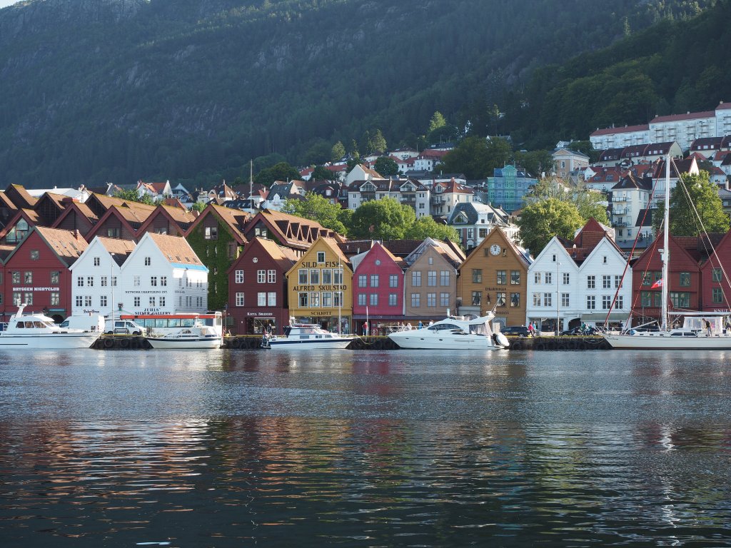
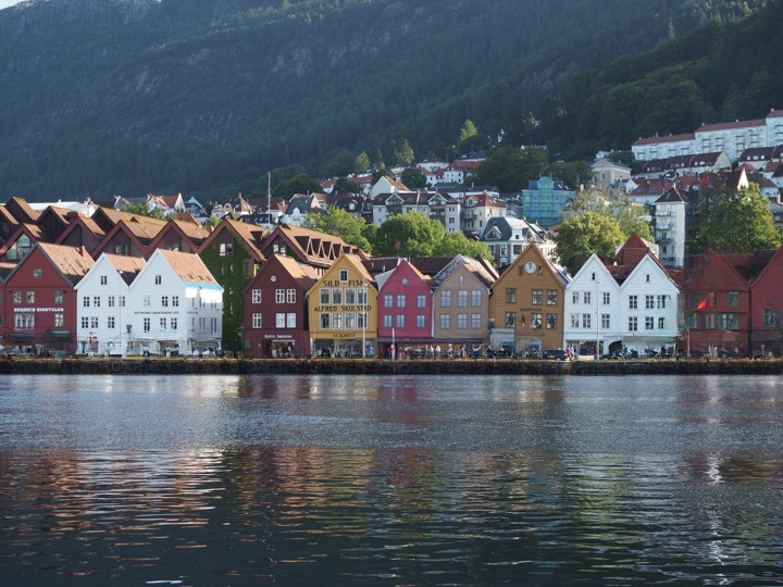
MYTH 13: Landscape photographs need good light.

REALITY: In reality there is no such thing as bad light, or bad weather, unless it is pouring. You can never guarantee what the weather will be like anywhere, and if you are travelling to places like Scotland, Iceland, or Norway the weather can change on the flip of a coin. There can be a lot of drizzle, or fog. You have to learn to make the most the situation, exploiting any kind of light.

MYTH 14: Manual exposure produces the best images.

REALITY: Many photographers use aperture-priority, or the oft-lauded P-mode. If you think something will be over- or under-exposed, then use exposure-bracketing. Modern cameras have a lot of technology to deal with taking optimal photographs, so don’t feel bad about using it.

MYTH 15: The fancy camera features are cool.

REALITY: No, they aren’t. Sure, try the built-in filters. They may be fun for a bit, but filters can always be added later. If you want to add filters, try posting to Instagram. For example, high-resolution mode is somewhat fun to play with, but it will eat battery life.

MYTH 16: One camera is enough.

REALITY: I never travel with less than two cameras, a primary, and a secondary, smaller camera, one that fits inside a jacket pocket easily (in my case a Ricoh GR III). There are risks when you are somewhere on vacation and your main camera stops working for some reason. A backup is always great to have, both for breakdowns, lack of batteries, or just for shooting in places where you don’t want to drag a bigger camera along, or would prefer a more inconspicuous photographic experience, e.g. museums, art galleries.

MYTH 17: More megapixels are better.

REALITY: I think optimally, anything from 16-26 megapixels is good. You don’t need 50MP unless you are going to print large posters, and 12MP likely is not enough these days.

MYTH 18: Shooting in RAW is the best.

REALITY: Probably, but here’s the thing, for the amateur, do you want to spend a lot of time post-processing photos? Maybe not? Setting the camera to JPEG+RAW is the best of both worlds. There is the issue of JPEG editing being destructive and RAW not.

MYTH 19: Backpacks offer the best way of carrying equipment.

REALITY: This may be true getting equipment from A to B, but schlepping a backpack loaded with equipment around every day during the summer can be brutal. No matter the type, backpacks + hot weather = a sweaty back. They also make you stand out, just as much as a FF camera with a 300mm lens. Opt instead for a camera sling, such as one from Peak Design. It has a much lower form factor and with a non-FF camera offers enough space for the camera, an extra lens, and a few batteries and memory cards. I’m usually able to shove in the secondary camera as well. They make you seem much more incognito as well.

MYTH 20: Carrying a film-camera is cumbersome.

REALITY: Film has made a resurgence, and although I might not carry one of my Exakta cameras, I might throw a half-frame camera in my pack. On a 36-roll film, this gives me 72 shots. The film camera allows me to experiment a little, but not at the expense of missing a shot.

MYTH 21: Travel photos will be as good as those in photo books.

REALITY: Sadly not. You might be able to get some good shots, but the reality is those shots in coffee-table photo books, and on TV shows are done with much more time than the average person has on location, and with the use of specialized equipment like drones. You can get some awesome imagery with drones, especially for video, because they can get perspectives that a person on the ground just can’t. If you spend an hour at a place you will have to deal with the weather that exists – someone who spends 2-3 days can wait for optimal conditions.

MYTH 22: If you wait long enough, it will be less busy.

REALITY: Some places are always busy, especially so it if is a popular landmark. The reality is short of getting up at the crack of dawn, it may be impossible to get a perfect picture. A good example is Piazza San Marco in Venice… some people get a lucky shot in after a torrential downpour, or some similar event that clears the streets, but the best time is just after sunrise, otherwise it is swamped with tourists. Try taking pictures of lesser known things instead of waiting for the perfect moment.

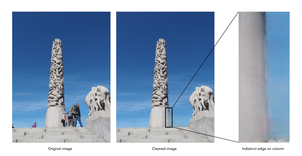
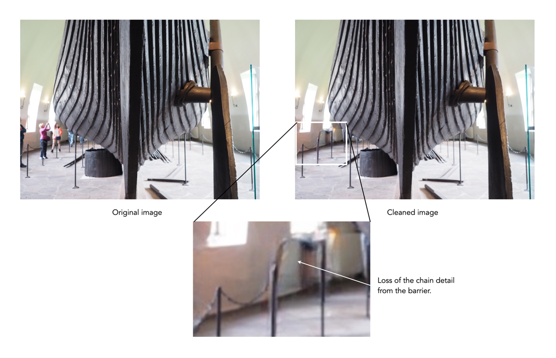
MYTH 23: Unwanted objects can be removed in post-processing.

REALITY: Sometimes popular places are full of tourists… like they are everywhere. In the past it was impossible to remove unwanted objects, you just had to come back at a quieter time. Now there are numerous forms of post-processing software like Cleanup-pictures that will remove things from a picture. A word of warning though, this type of software may not always work perfectly.

MYTH 24: Drones are great for photography.

REALITY: It’s true, drones make for some exceptional photographs, and video footage. You can actually produce aerial photos of scenes like the best professional photographers, from likely the best vantage points. However there are a number of caveats. Firstly, travel drones have to be a reasonable size to actually be lugged about from place to place. This may limit the size of the sensor in the camera, and also the size of the battery. Is the drone able to hover perfectly still? If not, you could end up with somewhat blurry images. Flight time on drones is usually 20-30 minutes, so extra batteries are a requirement for travel. The biggest caveat of course is where you can fly drones. For example in the UK, non-commercial drone use is permitted, however there are no-fly zones, and permission is needed to fly over World heritage sites such as Stonehenge. In Italy a license isn’t required, but drones can’t be used over beaches, towns or near airports.

A review of SKRWT – keystone correction for IOS

December 2, 2021 / spqr / Leave a comment

For a few years now, I have been using SKRWT, an app that does perspective correction in IOS.

The goal was to have some way of quickly fixing issues with perspective, and distortions, in photographs. The most common form of this is the keystone effect (see previous post) which occurs when the image plane is not parallel to the lines that are required to be parallel in the photograph. This usually occurs when taking photographs of buildings where we tilt the camera backwards, in order to include the whole scene. The building appears to be “falling away” from the camera. Fig.1 shows a photograph of a church in Montreal. Notice, the skew as the building seems to tilt backwards.

The process of correcting distortions with SKRWT is easy. Pick an image, and then a series of options are provided in the icon bar below the imported picture. The option that best approximates the types of perspective distortion is selected, and a new window opens, with a grid overlaid upon the image. A slider below the image can be used to select the magnitude of the distortion correction, with the image transformed as the slider is moved. When the image looks geometrically corrected, pressing the tick stores the newly corrected image.

Fig. 2: *The simple process of correcting a vertical distortion*

Using the SKRWT app, the perspective distortion can be fixed, but at a price. The problem is that correcting for the perspective distortion requires distorting the image, which means it will likely be larger than the original, and will need to be cropped (otherwise the image will contain black background regions).

Here is a third example, of Toronto’s flatiron building, with the building surrounded by enough “picture” to allow for corrective changes that don’t cut off any of the main object.

Overall the app is well designed and easy to use. In fact it will remove quite complex distortions, although there is some loss of content in the images processed. To use this, or any similar perspective correction software properly, you really have to frame the building with enough background to allow for corrections – not so you are left with half a building.

The sad thing about this app is something that plagues a lot of apps – it has become a zombie app. The developer was suppose to release version 1.5 in December 2020, but alas nothing has appeared, and the website has had no updates. Zombie apps work while the system they are on works, but upgrade the phone, or OS, and there is every likelihood it will no longer work.

Removing unwanted objects from pictures with Cleanup.pictures

November 18, 2021 / spqr / Leave a comment

Ever been on vacation somewhere, and wanted to take a picture of something, only to be thwarted by the hordes of tourists? Typically for me it’s buildings of architectural interest, or wide-angle photos in towns. It’s quite a common occurrence, especially in places where tourists tend to congregate. There aren’t many choices – if you can come back at a quieter time that may be the best approach, but often you are at a place for a limited time-frame. So what to do?

Use software to remove the offending objects, or people. Now this type of algorithm designed to remove objects from an image has been around for about 20 years, known in the early years as digital inpainting, akin to the conservation process where damaged, deteriorating, or missing parts of an artwork are filled in to present a complete image. In its early forms digital inpainting algorithms worked well in scenes where the object to be removed was surrounded by fairly uniform background, or pattern. In complex scenes they often didn’t fair so well. So what about the newer generation of these algorithms?

There are many different types of picture cleaning software, some stand-alone such as the AI-powered IOS app Inpaint, others in the form of features in photo processing software such as Photoshop. One new-comer to the scene is web-based, open-source, Cleanup.pictures. It is incredibly easy to use. Upload a picture, choose the size of the brush tool, paint over the unwanted object with the brush tool, and voila! a new image, sans the offending object. Then you can just download the “cleaned” image. So how well does it work? Below are some experiments.

The first image is a vintage photograph of Paris, removing all the people from the streets. The results are actually quite exceptional.

The second image is a photograph taken in Glasgow, where the people and passing car have been erased.

The third image is from a trip to Norway, specifically the harbour in Bergen. This area always seems to have both people and boats, so it is hard to take clear pictures of the historical buildings.

The final image is a photograph taken by Prokudin-Gorskii Collection at the Library of Congress. The image is derived from a series of glass plates, and suffers from some of the original glass plates being broken, with missing pieces of glass. The result of cleaning up the image, actually has done a better job than I could ever have imagined.

The AI used in this algorithm is really good at what it does, like *really good*, and it is easy to use. You just keep cleaning up unwanted things until you are happy with the result. The downsides? It isn’t exactly perfect all the time. In regions to be removed where there are fine details you want to retain, they are often removed. Sometimes areas become “soft” because they have to be “created” because they were obscured by objects before – especially prevalent in edge detail. Some examples are shown below:

Creation of detail during inpainting

It only produces low-res images, with a maximum width of 720 pixels. You can upgrade to the Pro version to increase resolution (2K width). It would be interesting to see this algorithm produce large scale cleaned images. There is also the issue of uploading personal photos to a website, although they do make the point of saying that images are discarded once processed.

For those interested in the technology behind the inpainting, it is based on an algorithm known as large mask inpainting, developed by a group at Samsung, and associates [1]. The code can be obtained directly from github for those who really want to play with things.

Suvorov, R., et al. Resolution-robust Large Mask Inpainting with Fourier Convolutions (2022)

Demystifying Colour (viii) : CIE colour model

November 17, 2021 / spqr / Leave a comment

The Commission Internationale de l’Eclairage (French for International Commission on Illumination) , or CIE is an organization formed in 1913 to create international standards related to light and colour. In 1931, CIE introduced CIE1931, or CIEXYZ, a colorimetric colour space created in order to map out all the colours that can be perceived by the human eye. CIEXYZ was based on statistics derived from extensive measurements of human visual perception under controlled conditions.

In the 1920s, colour matching experiments were performed independently by physicists W. David Wright and John Guild, both in England [2]. The experiments were carried out with 7 (Guild) and 10 (Wright) people. Each experiment involved a subject looking through a hole which allowed for a 2° field of view. On one side was a reference colour projected by a light source, while on the other were three adjustable light sources (the primaries were set to R=700.0nm, G=546.1nm, and B=435.8nm.). The observer would then adjust the values of three primary lights until they can produce a colour indistinguishable from a reference light. This was repeated for every visible wavelength. The result of the colour-matching experiments was a table of RGB triplets for each wavelength. These experiments were not about describing colours with qualities like hue and saturation, but rather just attempt to explain how combinations of light appear to be the same colour to most people.

Fig.1: An example of the experimental setup of Guild/Wright

In 1931 CIE amalgamated Wright and Guild’s data and proposed two sets of of colour matching functions: CIE RGB and CIE XYZ. Based on the responses in the experiments, values were plotted to reflect how the average human eye senses the colours in the spectrum, producing three different curves of intensity for each light source to mix all colours of the colour spectrum (Figure 2), i.e. Some of the values for red were negative, and the CIE decided it would be more convenient to work in a colour space where the coefficients were always positive – the XYZ colour matching functions (Figure 3). The new matching functions had certain characteristics: (i) the new functions must always be greater than or equal to zero; (ii) the y function would describe only the luminosity, and (iii) the white-point is where x=y=z=1/3. This produced the CIE XYZ colour space, also known as CIE 1931.

Fig.2: *CIE RGB colour matching function*s

Fig.3: *CIE XYZ colour matching functions*

The CIE XYZ colour space defines a quantitative link between distributions of wavelengths in the electromagnetic visible spectrum, and physiologically perceived colours in human colour vision. The space is based on three fictional primary colours, X, Y, and Z, where the Y component corresponds to the luminance (as a measure of perceived brightness) of a colour. All the visible colours reside inside an open cone-shaped region, as shown in Figure 4. CIE XYZ is then a mathematical generalization of the colour portion of the HVS, which allows us to define colours.

Fig.4: *CIE XYZ colour space* (G denotes the axis of neutral gray).

The luminance in XYZ space increases along the Y axis, starting at 0, the black point (X=Y=Z=0). The colour hue is independent of the luminance, and hence independent of Y. CIE also defines a means of describing hues and saturation, by defining three normalized coordinates: x, y, and z (where x+y+z=1).

x = X / (X+Y+Z)
y = Y / (X+Y+Z)
z = Z / (X+Y+Z)
z = 1 - x - y

The x and y components can then be taken as the chromaticity coordinates, determining colours for a certain luminance. This system is called CIE xyY, because a colour value is defined by the chromaticity coordinates x and y in addition to the luminance coordinate Y. More on this in the next post on chromaticity diagrams.

The RGB colour space is related to XYZ space by a linear coordinate transformation. The RGB colour space is embedded in the XYZ space as a distorted cube (see Figure 5). RGB can be mapped onto XYZ using the following set of equations:

X = 0.41847R - 0.09169G - 0.0009209B
Y = -0.15866R + 0.25243G - 0.0025498B (luminance)
Z = -0.082835R + 0.015708G + 0.17860B

CIEXYZ is non-uniform with respect to human visual perception, i.e. a particular fixed distance in XYZ is not perceived as a uniform colour change throughout the entire colour space. CIE XYZ is often used as an intermediary space in determining a perceptually uniform space such as CIE Lab (or Lab), or CIE LUV (or Luv).

CIE 1976 CIEL*u*v*, or CIELuv, is an easy to calculate transformation of CIE XYZ which is more perceptually uniform. Luv was created to correct the CIEXYZ distortion by distributing colours approximately proportional to their perceived colour difference.
CIE 1976 CIEL*a*b*, or CIELab, is a perceptually uniform colour differences and L* lightness parameter has a better correlation to perceived brightness. Lab remaps the visible colours so that they extend equally on two axes. The two colour components a* and b* specify the colour hue and saturation along the green-red and blue-yellow axes respectively.

In 1964 another set of experiments were done allowing for a 10° field of view, and are known as the CIE 1964 supplementary standard colorimetric observer. CIE XYZ is still the most commonly used reference colour space, although it is slowly being pushed to the wayside by CIE1976. There is a lot of information on CIE XYZ and its derivative spaces. The reader interested in how CIE1931 came about in referred to [1,4]. CIELab is the most commonly used CIE colour space for imaging, and the printing industry.

How does high-resolution mode work?

November 1, 2021 / spqr / Leave a comment

One of the tricks of modern digital cameras is a little thing called “high-resolution mode” (HRM), which is sometimes called pixel-shift. It effectively boosts the resolution of an image, even though the number of pixels used by the camera’s sensor does not change. It can boost a 24 megapixel image into a 96 megapixel image, enabling a camera to create images at a much higher resolution than its sensor would normally be able to produce.

So how does this work?

In normal mode, using a colour filter array like Bayer, each photosite acquires one particular colour, and the final colour of each pixel in an image is achieved by means of demosaicing. The basic mechanism for HRM works through sensor-shifting (or pixel-shifting) i.e. taking a series of exposures and processing the data from the photosite array to generate a single image.

An exposure is obtained with the sensor in its original position. The exposure provides the first of the RGB components for the pixel in the final image.
The sensor is moved by one photosite unit in one of the four principal directions. At each original array location there is now another photosite with a different colour filter. A second exposure is made, providing the second of the components for the final pixel.
Step 2 is repeated two more times, in a square movement pattern. The result is that there are four pieces of colour data for every array location: one red, one blue, and two greens.
An image is generated with each RGB pixel derived from the data, the green information is derived by averaging the two green values.

No interpolation is required, and hence no demosaicing.

*The basic high-resolution mode process (the arrows represent the direction the sensor shifts)*

In cameras with HRM, it functions using the motors that are normally dedicated to image stabilization tasks. The motors effectively move the sensor by exactly the amount needed to shift the photosites by one whole unit. The shifting moves in such a manner that the data captured includes one Red, one Blue and two Green photosites for each pixel.

There are many benefits to this process:

The total amount of information is quadrupled, with each image pixel using the actual values for the colour components from the correct physical location, i.e. full RGB information, no interpolation required.
Quadrupling the light reaching the sensor (four exposures) should also cut the random noise in half.
False-colour artifacts often arising in the demosaicing process are no longer an issue.

There are also some limitations:

It requires a very steady scene. It doesn’t work well if the camera is on a tripod, yet there is a slight breeze, moving the leaves on a tree.
It can be extremely CPU-intensive to generate a HRM RAW image, and subsequently drain the battery. Some systems, like Fuji’s GFX100 uses off-camera, post-processing software to generate the RAW image.

Here are some examples of the high resolution modes offered by camera manufacturers:

Fujifilm – Cameras like the GFX100 (102MP) have a Pixel Shift Multi Shot mode where the camera moves the image sensor by 0.5 pixels over 16 images and composes a 400MP image (yes you read that right).
Olympus – Cameras like the OM-D E-M5 Mark III (20.4MP), has a High-Resolution Mode which takes 8 shots using 1 and 0.5 pixel shifts, which are merged into a 50MP image.
Panasonic – Cameras like the S1 (24.2MP) have a High-Resolution mode that results in 96MP images. The Panasonic S1R at 47.3MP produces 187MP images.
Pentax – Cameras like the K-1 II (36.4MP) use a Pixel Shift Resolution System II with a Dynamic Pixel Shift Resolution mode (for handheld shooting).
Sony – Cameras like the A7R IV (61MP) uses a Pixel Shift Multi Shooting mode to produce a 240MP image.

Do you need 61 megapixels, or even 102?

October 27, 2021February 21, 2023 / spqr / Leave a comment

The highest “native” resolution camera available today is the Phase One FX IQ4 medium format camera at 150MP. Higher than that there is the Hasselblad H6D-400C at 400MP, but it uses pixel-shift image capture. Next in line is the medium format Fujifilm GFX 100/100S at 102 MP. In fact we don’t get to full-frame sensors until we hit the Sony A7R IV, at a tiny 61MP. Crazy right? The question is how useful are these sensors for the photographer? The answer is not straightforward. For some photographic professionals these large sensors make inherent sense. For the average casual photographer, they likely don’t.

People who don’t photograph a lot tend to be somewhat bamboozled by megapixels, like more is better. But more megapixels does not mean a better image. Here are some things to consider when thinking about when considering megapixels.

Sensor size

There is a point when it becomes hard to cram any more photosites into a particular sensor – they just become too small. For example the upper bound with APC-S sensors seems to be around 33MP, with full-frame it seems to be around 60MP. Put too many photosites on a sensor and the density of the photosites increases, as the size of the photosites decreases. The smaller the photosite, the harder it is for it to collect light. For example Fuji APS-C cameras seem to tap out at around 26MP – the X-T30 has a photosite pitch of 3.75µm. Note that Fuji’s leap to a larger number of megapixels also means a leap to a larger sensor – the medium format sensor with a sensor size of 44×33mm. Compared to the APS-C sensor (23.5×15.6mm), the medium format sensor is nearly four times the size. A 51MP medium format sensor has photosites which are 5.33µm in size, or 1.42 times of size of the 26MP APS-C sensor.

The verdict? Squeezing more photosites onto the same size sensor does increase resolution, but sometimes at the expense of how light is acquired by the sensor.

Image and linear resolution

Sensors are made up of photosites that acquire the data used to make image pixels. The image resolution of an image describes the number of pixels used to construct an image. For example a 16MP sensor with a 3:2 aspect ratio has an image resolution of 4899×3266 pixels – the dimensions are sometimes termed the linear resolution. To obtain twice the image resolution we need a 64MP sensor, rather than a 32MP sensor. A 32MP sensor has 6928×4619 photosites, which results in a 1.4 times increase in the linear resolution of the image. The pixel count has doubled, but the linear resolution has not. Upgrading from a 16MP sensor to a 24MP sensor means a ×1.5 increase in the pixel count, and a ×1.2 increase in linear resolution. The transition from 16MP to 64MP is a ×2 increase in linear resolution, and a ×4 increase in the number of pixels. That’s why the difference between 16MP and 24MP sensors is also dubious (see Figure 1).

Fig.1: *Different* *image resolutions and megapixels within an APS-C sensor*

To double the linear resolution of a 24MP sensor you need a 96MP sensor. So the 61MP sensor provides about double the linear resolution of a 16MP sensor, as the 102MP sensor doubles the 24MP sensor.

The verdict? Doubling the pixel count, i.e. image resolution, does not double the linear resolution.

Photosite size

When you have more photosites, you also have to ask what their physical size is. Squeezing 41 million photosites on the same size sensor as one which previously had 24 million pixels means that each pixel will be smaller, and that comes with its own baggage. Consider for instance the full-frame camera, the full-frame Leica M10-R, which has a 7864×5200 photosites (41MP) meaning the photosite size is roughly 4.59 microns. The full-frame 24MP Leica M-E has a photosite size of 5.97 microns, so 1.7 times the area. Large photosites allow more light to be captured, while smaller photosites gather less light, so when their low signal strength is transformed into a pixel, more noise is generated.

The verdict? From the perspective of photosite size, 24MP captured on a full-frame sensor will be better than 24MP on an APS-C sensor, which in turn is better than 24MP on a M43 sensor (theoretically anyways).

Optics

Comparing the quality of a 16MP lens to a 24MP lens, we might determine that the quality, and sharpness of the lens is more important than the number of pixels. In fact too many people place an emphasis on the number of pixels and forget about the fact that light has to pass through a lens before it is captured by the sensor and converted into an image. Many high-end cameras already provide an in-camera means of generating a high-resolution images, often four times the actual image resolution – so why pay more for more megapixels? Is a 50MP full-frame sensor any good without optically perfect (or near-perfect) lenses? Likely not.

The verdict? Good quality lenses are just as important as more megapixels.

File size

People tend to forget that images have to be saved on memory cards (and post-processed). The greater the megapixels, the greater the resulting file size. A 24MP image stored as a 24-bit/pixel JPEG will be 3.4MB in size (at 1/20). As a 12-bit RAW the file size would be 34MB. A 51MP camera like the Fujifilm GFX 50S II would have a 7.3MB JPEG, and a 73MB 12-bit RAW. If the only format used is JPEG it’s probably, fine, but the minute you switch to RAW it will use way more storage.

The verdict? More megapixels = more megabytes.

Camera use

The most important thing to consider may be what the camera is being used for?

Website / social media photography – Full-width images for websites are optimal at around 2400×1600 (aka 4MP), blog-post images max. 1500 pixels in width (regardless of height), and inside content max 1500×1000. Large images can reduce website performance, and due to screen resolution won’t be visualized to their fullest capacity anyways.
Digital viewing – 4K televisions have roughly 3840×2160 = 8,294,400 pixels. Viewing photographs from a camera with a large spatial resolution will just mean they are down-sampled for viewing. Even the Apple Pro Display XDR only has 6016×3384=20MP view capacity (which is a lot).
Large prints – Doing large posters, for example 20×30″ requires a good amount of resolution if they are being printed at 300DPI, which is the nominal standard. So this needs about 54MP (check out the calculator). But you can get by with less resolution because few people view a poster at 100%.
Average prints – An 8×10″ print requires 2400×3000 = 7.2MP at 300DPI. A 26MP image will print maximum size 14×20″ at 300DPI (which is pretty good).
Video – Does not need high resolution, but rather 4K video at a descent frame rate.

The verdict? The megapixel amount really depends on the core photographic application.

Postscript

So where does that leave us? Pondering a lot of information, most of which the average photographer may not be that interested in. Selecting the appropriate megapixel size is really based on what a camera will be used for. If you commonly take landscape photographs that are used in large scale posters, then 61 or 102 megapixels is certainly not out of the ballpark. For the average photographer taking travel photos, or for someone taking images for the web, or book publishing, then 16MP (or 24MP at the higher end) is ample. That’s why smartphone cameras do so well at 12MP. High MP cameras are really made more for professionals. Nobody needs 61MP.

The overall erdict? Most photographers don’t need 61 megapixels. In reality anywhere between 16 and 24 megapixels is just fine.

Photosites – Quantum efficiency

October 15, 2021 / spqr / Leave a comment

Not every photo that makes it through the lens ends up in a photosite. The efficiency with which photosites gather incoming light photons is called its quantum efficiency (QE). The ability to gather light is determined by many factors including the micro lenses, sensor structure, and photosite size. The QE value of a sensor is a fixed value that depends largely on the chip technology of the sensor manufacturer. The QE is averaged out over the entire sensor, and is expressed as the chance that a photon will be captured and converted to an electron.

*Quantum efficiency* (P = Photons per μm², e = electrons)

The QE is a fixed value and is dependent on a sensor manufacturers design choices. The QE is averaged out over the entire sensor. A sensor with an 85% QE would produce 85 electrons of signal if it were exposed to 100 photons. There is no way to effect the QE of a sensor, i.e. you can’t change things by changing the ISO.

The QE is typically 30-55% meaning 30-55% of the photons that fall on any given photosite are converted to electrons. (front illuminated sensors). In back illuminated sensors, like those typically found on smartphones, the QE is approximately 85%. The website Photons to Photos has a list of sensor characteristics for a good number of cameras. For example the sensor in my Olympus OM-D E-M5 Mark II has a supposed QE of 60%. Trying to calculate the QE of a sensor in non-trivial.

Fixing the “crop-factor” issue

July 29, 2021 / spqr / 3 Comments

We use the term “cropped sensor” only due to the desire to describe a sensor in terms of the 35mm standard. It is a relative term which compares two different types of sensor, but it isn’t really that meaningful. Knowing that a 24mm MFT lens “behaves” like a 48mm full-frame lens is pointless if you don’t understand how a 48mm lens behaves on a full-frame camera. All sensors could be considered “full-frame” in the context of their environment, i.e. a MFT camera has a full-frame sensor as it relates to the MFT standard.

As mentioned in a previous post, the “35mm equivalence” is used to relate a crop-factor lens to its full-frame equivalent. The biggest problem with this is the amount of confusion it creates for novice photographers. Especially as focal lengths on lenses are always the same, yet the angle-of-view changes according to the sensor. However there is a solution to the problem, and that is to stop using the focal length to define a lens, and instead use AOV. This would allow people to pick a lens based on its angle-of view, both in degrees, but also from a descriptive point of view. For example, a wide angle lens in full-frame is 28mm – its equivalent in APS-C in 18mm, and MFT is 14mm. It would be easier just to label these by the AOV as “wide-74°”.

It would be easy to categorize lenses into six core groups based on horizontal AOV (diagonal AOV in []) :

Ultra-wide angle: 73-104° [84-114°]
Wide-angle: 54-73° [63-84°]
Normal (standard): 28-54° [34-63°]
Medium telephoto: 20-28° [24-34°]
Telephoto: 6-20° [8-24°]
Super-telephoto: 3-6° [4-8°]

*Lenses could be advertised using a graphic to illustrate the AOV (horizontal) of the lens. This effectively removes the need to talk about focal length.*

They are still loosely based on how AOV related to 35mm focal lengths. For example 63° relates to the AOV of a 35mm lens, however it no longer really relates to the focal length directly. A “normal-40°” lens would be 40° no matter the sensor size, even though the focal lengths would be different (see table below). The only lenses left out of this are fish-eye lenses, which in reality are not that common, and could be put into a
specialty lens category, along with tilt-shift etc.

*Instead of brochures containing focal lengths they could contain the AOV’s.*

I know most lens manufacturers describe AOV using diagonal AOV, but this is actually more challenging for people to perceive, likely because looking through a camera we generally look at a scene from side-to-side, not corner-to-corner.

AOV	98°	84°	65°
MFT	8mm	10mm	14mm
APS-C	10mm	14mm	20mm
FF	16mm	20mm	28mm

Wide/ultra-wide angle lenses

AOV	54°	49°	40°
MFT	17mm	20mm	25mm
APS-C	24mm	28mm	35mm
FF	35mm	40mm	50mm

Normal lenses

AOV	28°	15°	10°
MFT	35mm	70mm	100mm
APS-C	45mm	90mm	135mm
FF	70mm	135mm	200mm

Telephoto lenses

Crafting Pixels

Vintage lenses, photography and digital imagery

digital photography