Sometimes algorithms talk about the mean or variance of a region of an image (sometimes called a neighbourhood, or window). But what does this refer to? The mean is the average of a series of numbers, and the variance measures the average degree to which each number is different from the mean. So the mean of a 3×3 pixel neighbourhood is average of the 9 pixels within it, and the variance is the degree to which every pixel in the neighbourhood varies from the mean. To obtain a better perspective, it’s best to actually explore some images. Consider the grayscale image in Fig.1.
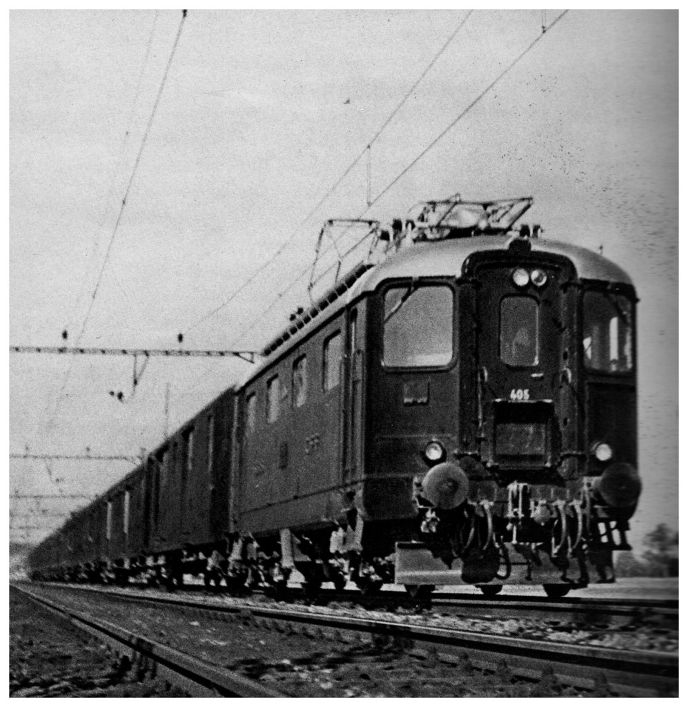
Four 200×200 regions have been extracted from the image, they are shown in Fig.2.
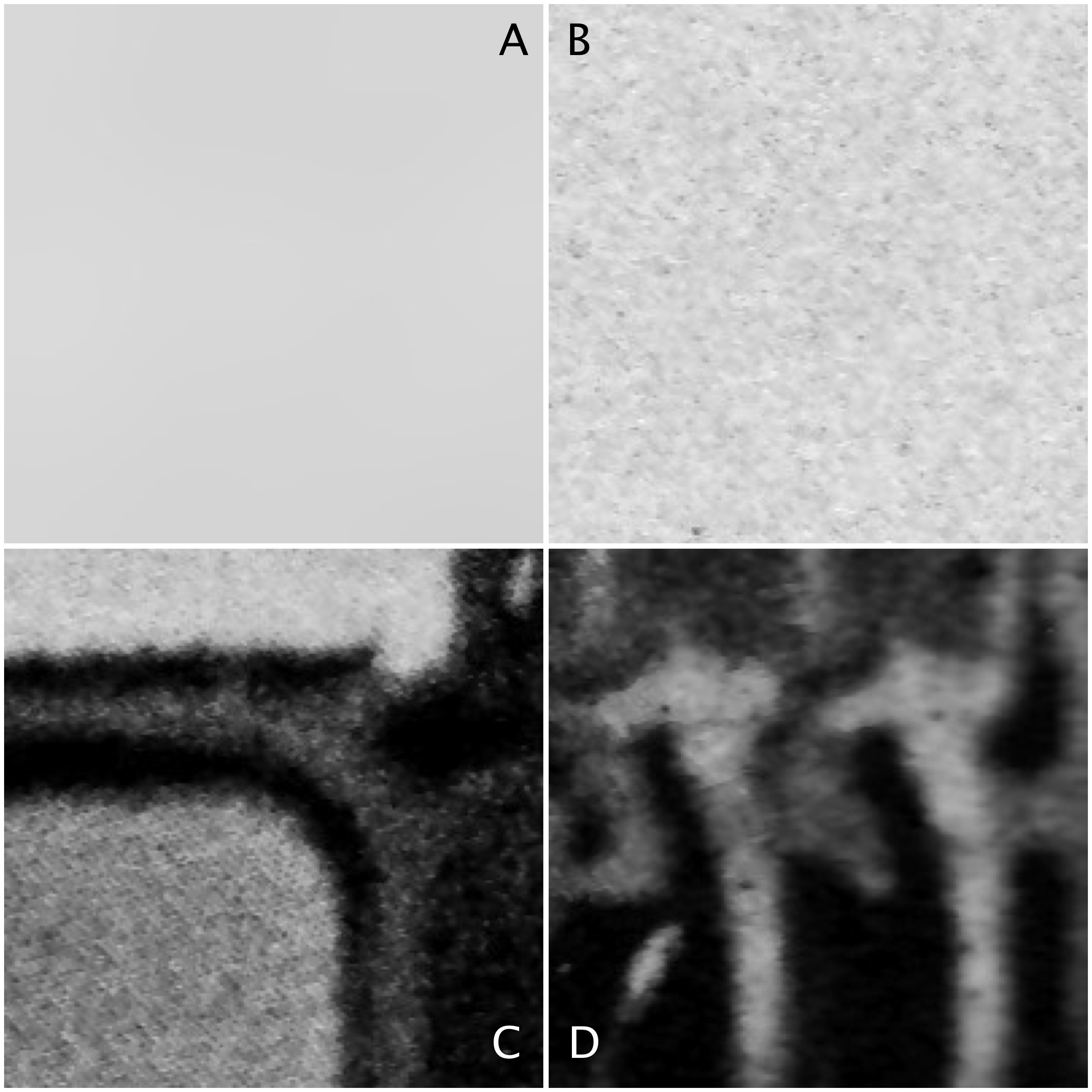
Statistics are given at the end of the post. Region B represents a part of the background sky. Region A is the same region processed using a median filter to smooth out discontinuities. In comparing region A and B, they both have similar means: 214.3 and 212.37 respectively. Yet their appearance is different – one is uniform, and the other seems to contain some variance, something we might attribute to noise in some circumstances. The variance of A is 2.65, versus 70.57 for B. Variance is a poor descriptive statistic, because it is hard to visualize, so many times it is converted to standard deviation (SD), which is just the square root of variance. For A and B, this is 1.63 and 8.4 respectively.
As shown in region C and D, more complex scenes introduce an increased variance, and SD. The variances can be associated with the distribution of the histograms shown below.
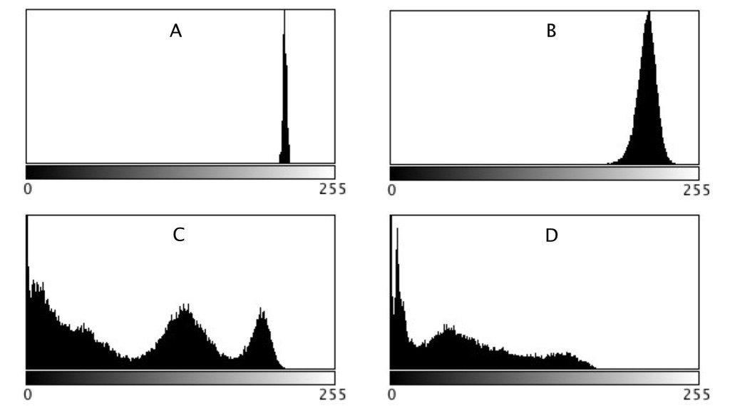
When comparing two regions, a lower variance (or in reality a lower SD) usually implies a more uniform region of pixels. Generally, mean and variance are not good estimators for image content because two totally different images can have same mean, and variance.
| Image | Mean | Variance | SD |
| A | 214.3 | 2.65 | 1.63 |
| B | 212.37 | 70.57 | 8.4 |
| C | 87.22 | 4463.11 | 66.81 |
| D | 56.33 | 2115.24 | 46.0 |
