This series of photographs and their associated histograms covers aesthetically pleasing bimodal histograms.
Histogram 1: A sky with texture
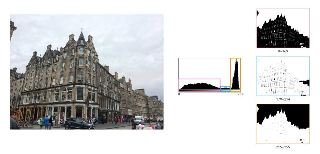
This image (of a building in Edinburgh) has a broad spectrum of intensity values. The histogram is bi-modal with two distinct humps. The right peak is associated with the overcast sky (and white van). The left shallow mound comprising both midtones and shadows makes up most of the remaining image content. There is a small flat region in between the two that makes up features like the lighter portions of the building. Note that pixels maps on the right of the histogram below show the associated pixels in black.
Histogram 2: Out on the lake
This photograph of the Kapellbrücke was taken in Lucerne, Switzerland. The histogram is bimodal, and asymmetric, and reflects the information in the image: the left hump (①) is associated with the lower portion of the image (shadows and midtones), and the right peak (② highlights) with the sky. There is relatively well contrasted image. The clouds have some good variation in colour, as opposed to begin pushed completely into the whites.
Fujifilm X10 (12MP): 7.1mm; f/9; 1/800
Histogram 3: Carved in stone
This is a photograph of the Lion of Lucerne, in Lucerne, Switzerland. It provides a classic asymmetric bimodal shaped histogram. The left mound, ①, contributes the images dark, shadowy regions, whereas the remaining, larger peak ②, bias towards highlights, defines most of the remaining image. It is well contrasted given that a shadow is cast on the sculpture as it is relief into the wall. The overlapping region between the two entities, ③, forms the transition regions from ① to ②, often visualized in the picture as regions of low “shadow”.
This series of photographs and their associated histograms covers good renditions of highlight clipping, i.e. photographs in which there are regions of white pixels, but they either genuinely exist in the image as white regions, or do not directly impact the aesthetics of the image.
Histogram 1: A bright overcast sky
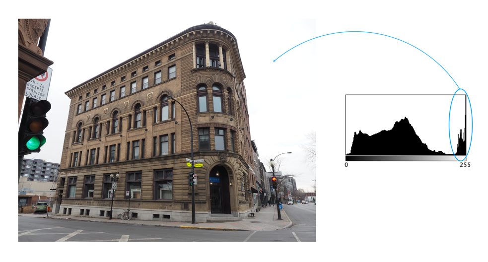
The image was taken on a very overcast day in Montreal. This is a good example of an image with highlight-clipping in the histogram, which is neither good nor bad. The building itself does not suffer from a lack of contrast, although the non-sky region can be enhanced slightly with no ill effects on the sky (because it is already basically white). This is a common situation in outdoor, overcast scenes. In an ideal world, more texture and contrast in the sky would be great, but in reality you have to use what nature provides.
Histogram 2: White buildings
This photograph was taken in Luzern, Switzerland. It is a well contrasted image, with a somewhat indistinct, multipeak histogram. The pixels are well distributed over the range of intensities, except for the spike at values 240-255. Here highlight clipping seems as though it has occurred because there are quite a number of white pixels in the image. However this density of white pixels comes not from anything being overblown, but rather from the white buildings in the image (of which there are many).
Fujifilm X10 (12MP): 7.1mm; f/4.5; 1/950
Histogram 3: A bit of overblown sky
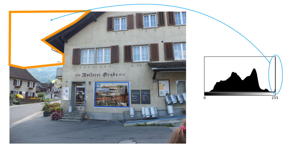
This photograph was taken in Grabs, Switzerland. The histogram is a nonuniform, and basically unimodal in shape, with the exception of a huge spike in the whites causing clipping. But this is a case of the highlight clipping not really affecting the core content of the image, i.e. it comprises the overblown sky in the top-left of the image. On a bright, partially overcast day, this is not an unusual scenario.
Understanding shape and tonal characteristics is part of the picture, but there are some other things about exposure that can be garnered from a histogram that are related to these characteristics. Remember, a histogram is merely a guide. The best way to understand an image is to look at the image itself, not just the histogram.
Contrast
Contrast is the difference in brightness between elements of an image, and can determine how dull or crisp an image appears with respect to intensity values. Note that the contrast described here is luminance or tonal contrast, as opposed to colour contrast. Contrast is represented as a combination of the range of intensity values within an image and the difference between the maximum and minimum pixel values. A well contrasted image typically makes use of the entire gamut of n intensity values from 0..n-1.
Image contrast is often described in terms of low and high contrast. If the difference between the lightest and darkest regions of an image is broad, e.g. if the highlights are bright, and the shadows very dark, then the image is high contrast. If an image’s tonal range is based more on gray tones, then the image is considered to have a low contrast. In between there are infinite combinations, and histograms where there is no distinguishable pattern. Figure 1 shows an example of low and high contrast on a grayscale image.
Fig.1: Examples of differing types of tonal contrast
The histogram of a high contrast image will have bright whites, dark blacks, and a good amount of mid-tones. It can often be identified by edges that appear very distinct. A low-contrast image has little in the way of tonal contrast. It will have a lot of regions that should be white but are off-white, and black regions that are gray. A low contrast image often has a histogram that appears as a compact band of intensities, with other intensity regions completely unoccupied. Low contrast images often exist in the midtones, but can also appear biased to the shadows or highlights. Figure 2 shows images with low and high contrast, and one which sits midway between the two.
Fig.2: Examples of low, medium, and high contrast in colour images
Sometimes an image will exhibit a global contrast which is different to the contrast found in different regions within the image. The example in Figure 3 shows the lack of contrast in an aerial photograph. The image histogram shows an image with medium contrast, yet if the image were divided into two sub-images, both would exhibit low-contrast.
Fig.3: Global contrast versus regional contrast
Clipping
A digital sensor is much more limited than the human eye in its ability to gather information from a scene that contains both very bright, and very dark regions, i.e. a broad dynamic range. A camera may try to create an image that is exposed to the widest possible range of lights and darks in a scene. Because of limited dynamic range, a sensor might leave the image with pitch-black shadows, or pure white highlights. This may signify that the image contains clipping.
Clipping represents the loss of data from that region of the image. For example a spike on the very left edge of a histogram may suggest the image contains some shadow clipping. Conversely, a spike on the very right edge suggests highlight clipping. Clipping means that the full extent of tonal data is not present in an image (or in actually was never acquired). Highlight clipping occurs when exposure is pushed a little too far, e.g. outdoor scenes where the sky is overcast – the white clouds can become overexposed. Similarly, shadow clipping means a region in an image is underexposed,
In regions that suffer from clipping, it is very hard to recover information.
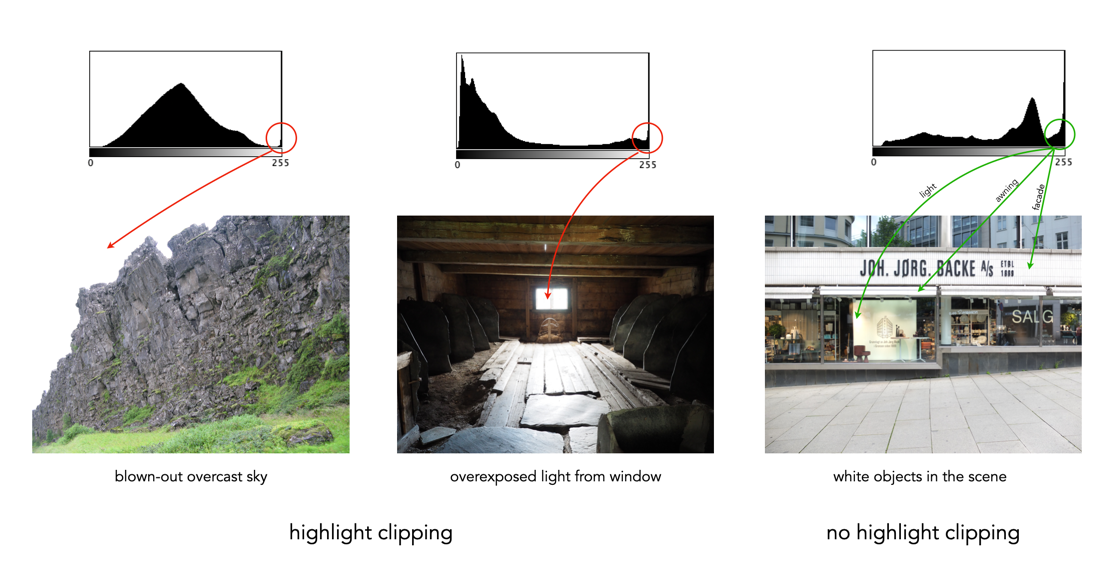
Fig.4: Shadow versus highlight clipping
Some describe the idea of clipping as “hitting the edge of the histogram, and climbing vertically”. In reality, not all histograms exhibiting this tonal cliff may be bad images. For example images taken against a pure white background are purposely exposed to produce these effects. Examples of images with and without clipping are shown in Figure 5.
Fig.5: Not all edge spikes in a histogram are clipping
Are both forms of clipping equally bad, or is one worse than the other? From experience, highlight clipping is far worse. That is because it is often possible to recover at least some detail from shadow clipping. On the other hand, no amount of post-processing will pull details from regions of highlight-clipping in an image.