Are-Bure-Boke aesthetic using the Provoke app

It is possible to experience the Are-Bure-Boke aesthetic in a very simple manner using the Provoke app. Developed by Toshihiko Tambo in collaboration with iPhoneography founder Glyn Evans, it was inspired by Japanese photographers of the late 1960’s like Daidō Moriyama, Takuma Nakahira and Yutaka Takanashi. This means it produces black and white images with the same gritty, grainy, blurry look reminiscent of the “Provoke” era of photography.

There isn’t much in the way of explanation on the app website, but it is fairly easy to use. There aren’t a lot of controls (the discussion below assumes the iPhone is held in landscape mode). The most obvious one is the huge red shutter release button. The button is obviously well proportioned in order to easily touch it, even though it does somewhat impede the use of the other option buttons. Two formats are provided: a square format 126 [1:1] and 35mm format 135 [3:2]. There is an exposure compensation setting which allows changes to be made up and down. The slider can be adjusted up to three stops in either direction: −3 to +3 in 1/3 steps. On the top-right is a button for the flash settings (Auto/On/Off). On the top-left there is a standard camera flip switch, and a preferences button which allows settings of Grid, TIFF, or GeoTag (all On/Off).

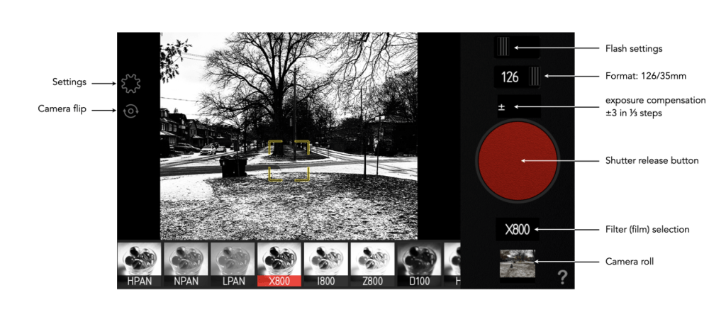
One of the things I dislike most about the app is related to its usability. Both the preferences and camera-flip buttons are very pale, making them hard to see in all but dark scenes when using 35mm format. The other thing I don’t particularly like is the inability to pull in a photograph from the camera roll. It is possible to access the camera roll to apply the B&W filters to photos on the camera roll, but the other functionality is restricted to live use. I do however like the fact that the app supports TIFF.

The original used to illustrate how the Provoke filters work (the “no filter” option).

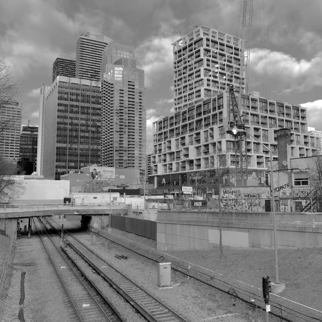
The app provides nine B&W filters, or rather “films” as the app puts it. They are in reality just filters, as they don’t seem to coincide with any panchromatic films that I could find. The first three options offer differing levels of contrast.

  • HPAN High Contrast – a high contrast film with fine grain.
  • NPAN Normal – normal contrast
  • LPAN Low Contrast – low contrast

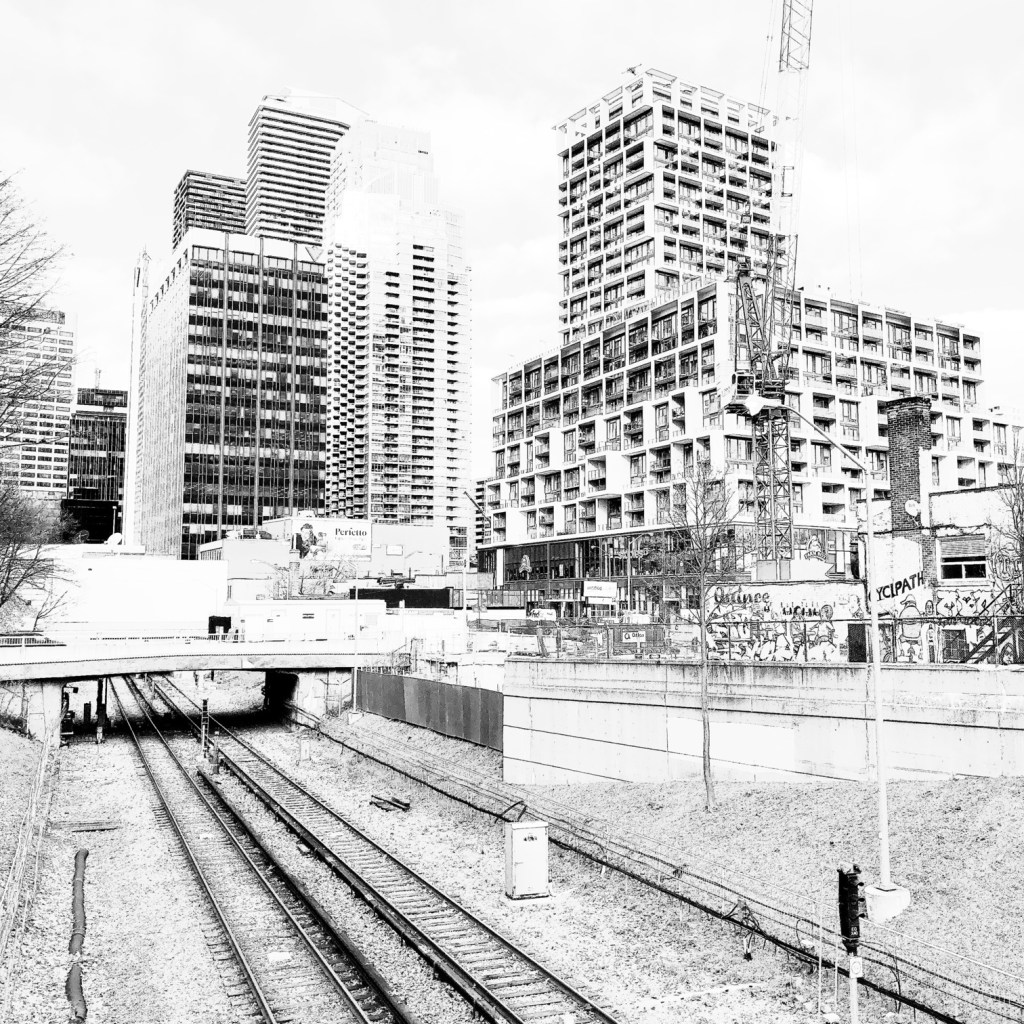
The next three are contrast + noise:

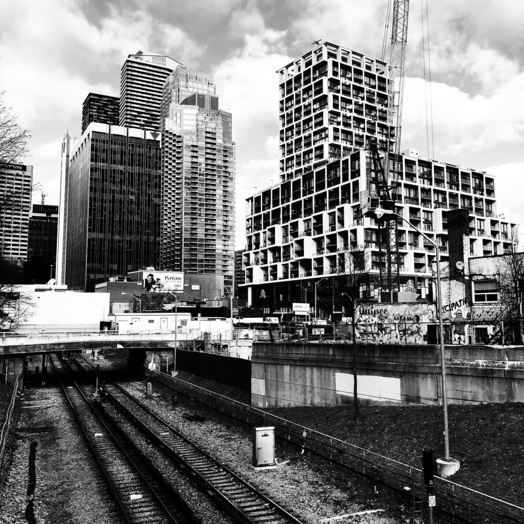
  • X800 – more High Contrast with more noise
  • I800 – IR like filter
  • Z800 – +2EV with more noise

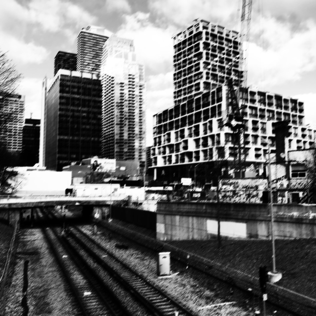
The film types with “100” designators introduce blur and grain.

  • D100 – Darken with Blur (4Pixel)
  • H100 – High Contrast with Blur(4Pixel)
  • E100 : +1.5EV with Blur(4Pixel)

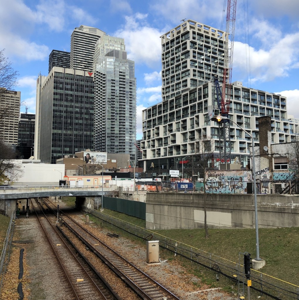
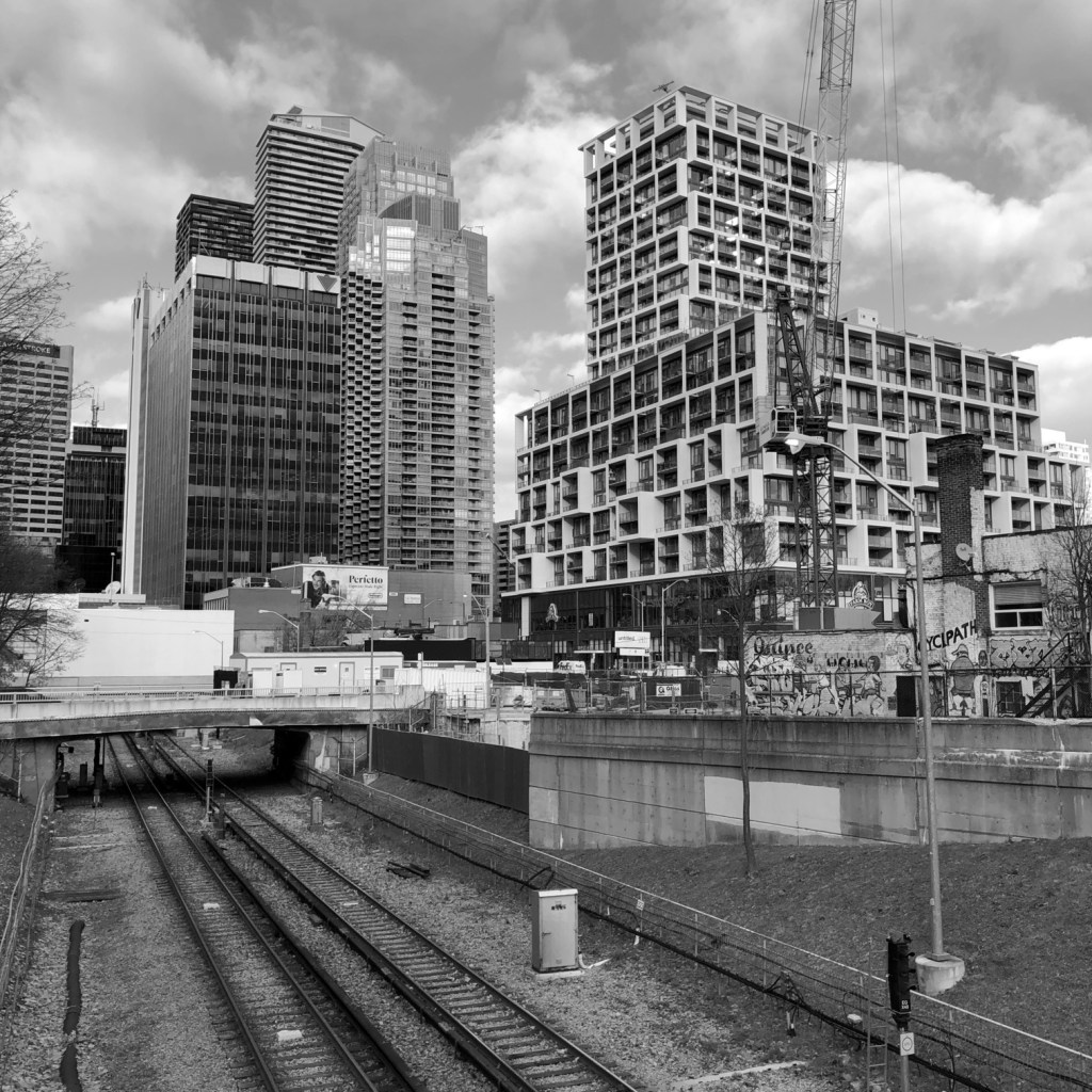
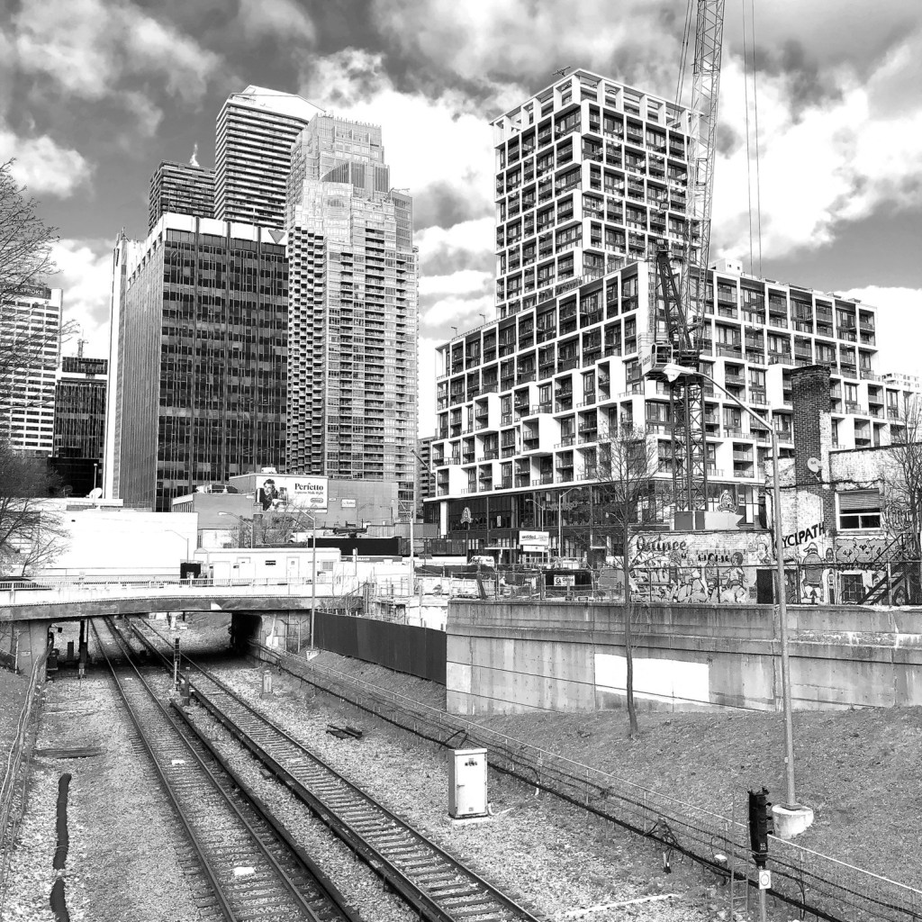
Examples of each of the filters are shown below. I have not adjusted any of the images for exposure compensation.

HPAN
X800
D100
NPAN
I800
H100
LPAN
Z800
E100

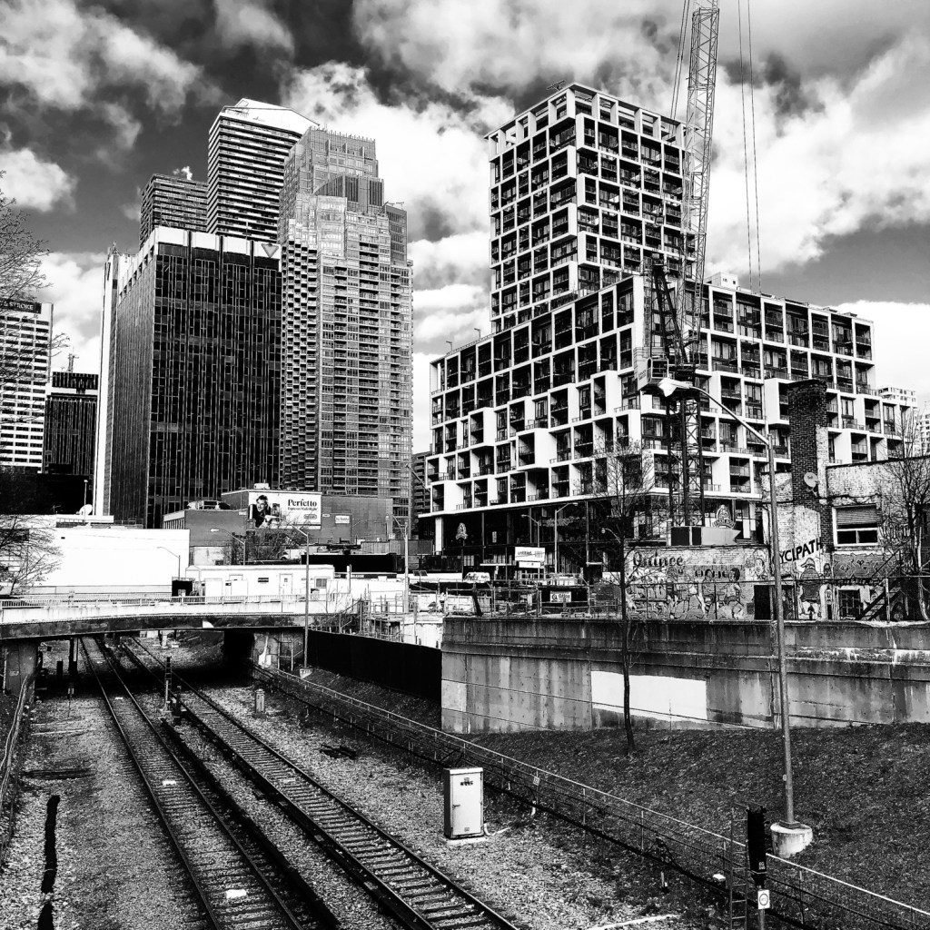
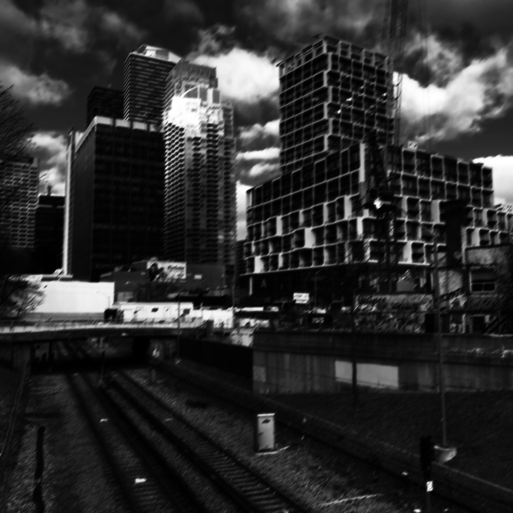
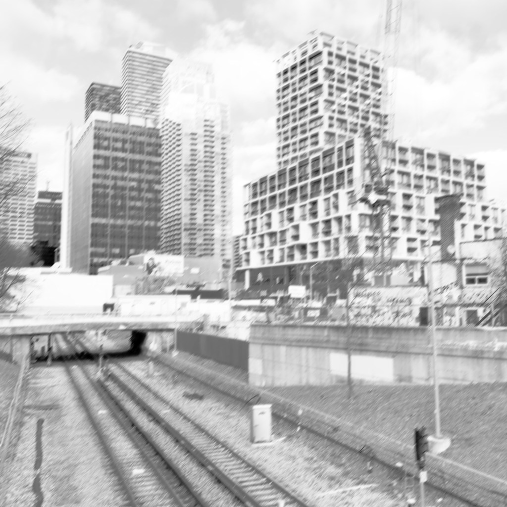
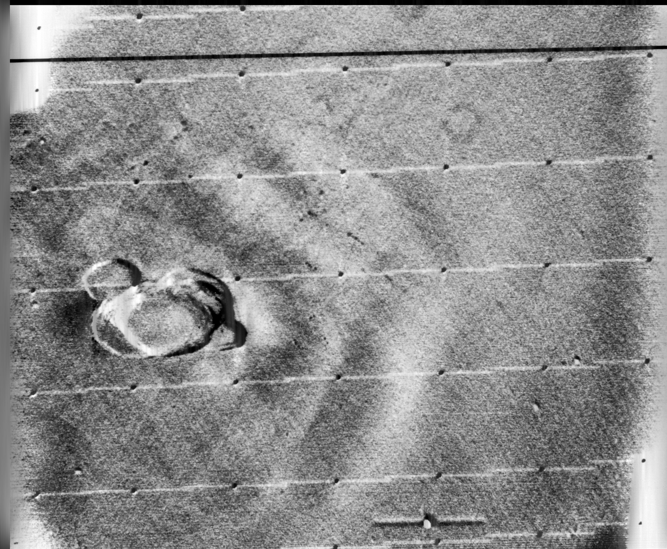
The Are-Bure-Boke aesthetic produces images which have characteristics of being grainy (Are), blurry (Bure) and out-of-focus (Boke). With the use of film cameras, these characteristics were intrinsic to the camera or film. The use of half-frame cameras allowed image grain to be magnified, low shutter speeds provide blur, and a fixed-focal length (providing a shallow DOF) provides out-of-focus. It is truly hard to replicate all these things in software. Contrast was likely added during the photo-printing stage.

What the app really lacks is the ability to specify a shutter-speed, meaning that Bure can not really be replicated. Blur is added by means of an algorithm, however is added across the whole image, simulating the entire camera panning across the scene using a low shutter speed, rather than capturing movement using a low-shutter speed (where some objects will not be blurred because they are stationary). It doesn’t seem like there is anything in the way of Boke, out-of-focus. Grain is again added by means of filter which adds noise. Whatever algorithm is used to replicate film grain also doesn’t work well, with uniform, high intensity regions showing little in the way of grain.

In addition Provoke also provides three colour modes, and a fourth no-filter option.

  • Nofilter
  • 100 Old Color
  • 100U Vivid and Sharp
  • 160N Soft
100
100U
160N

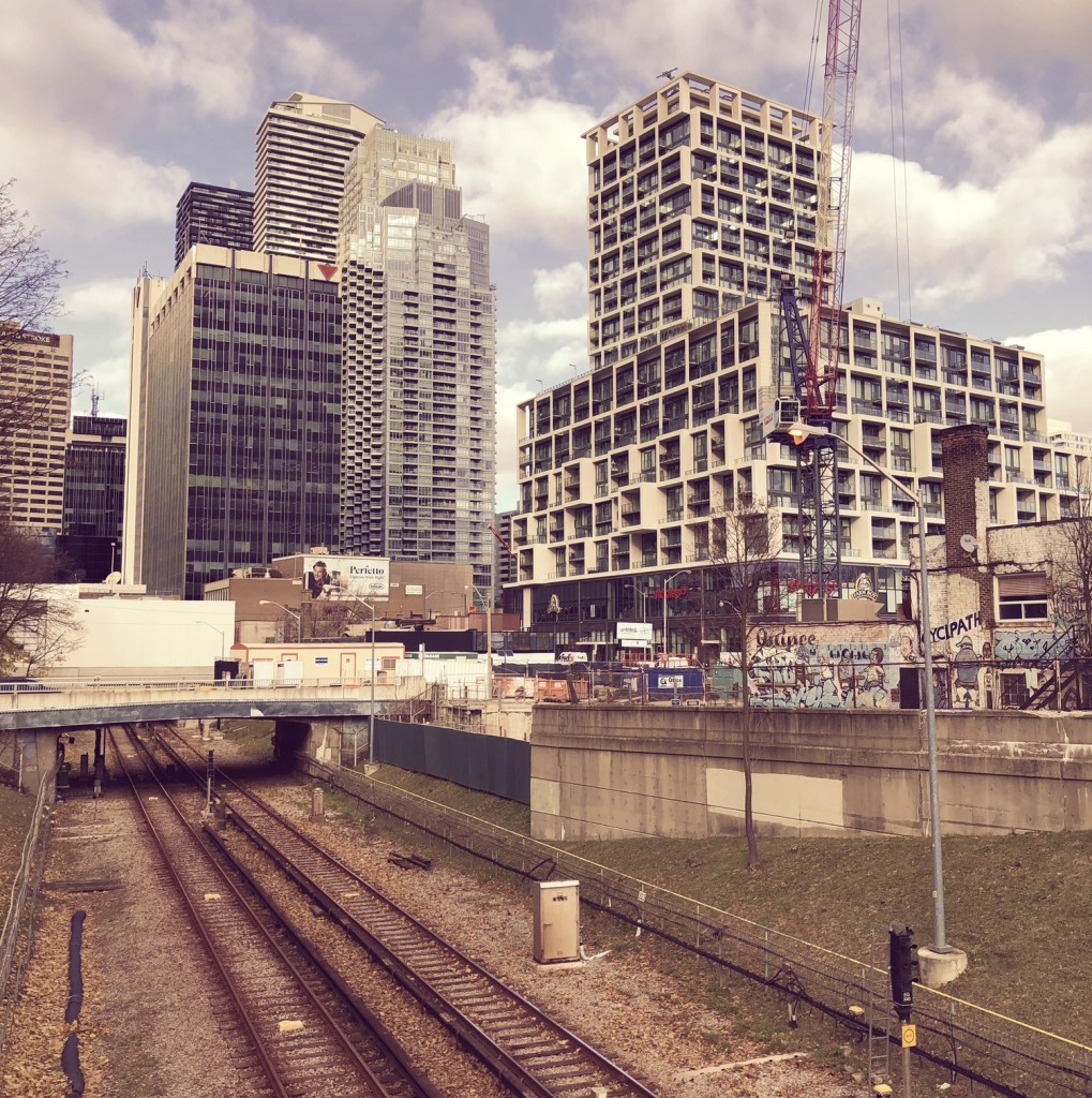
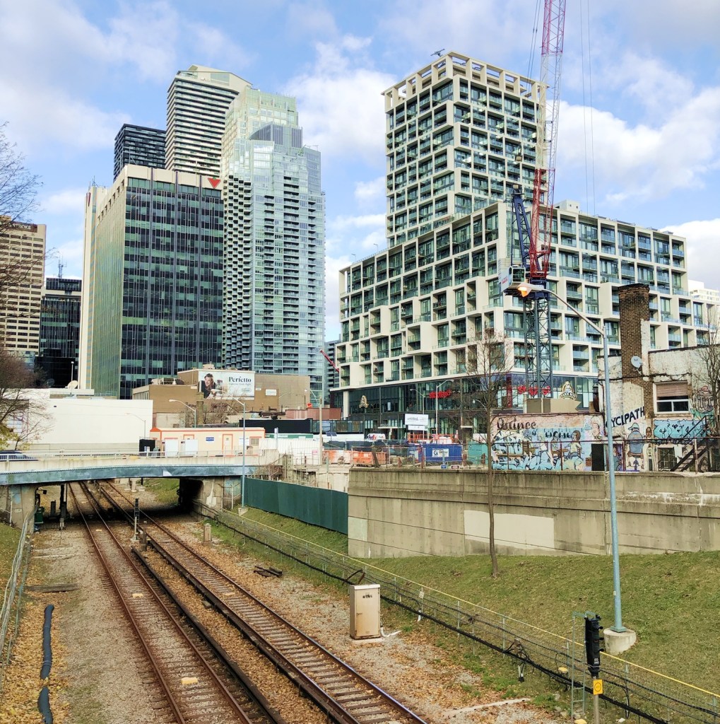
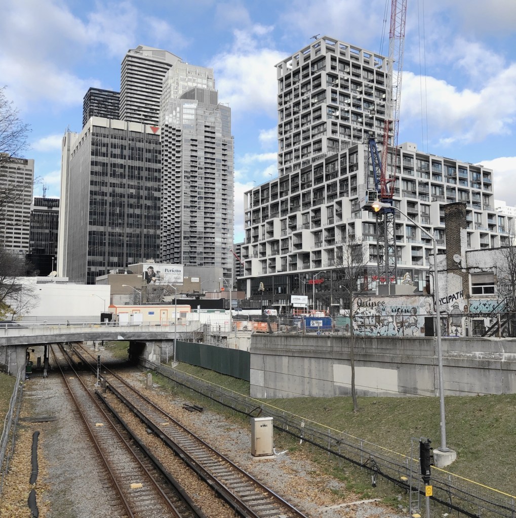
Honestly, I don’t know why these are here. Colour filters are a dime a dozen in just about every photo app… no need to crowd this app with them, although they are aesthetically pleasing. I rarely use anything except HPAN, and X800. Most of the other filters really don’t provide anything in the way of the contrast I am looking for, of course it depends on the particular scene. I like the app, I just don’t think it truly captures the point-and-shoot feel of the Provoke era.

The inherent difference between traditional Are-Bure-Boke vs the Provoke app is one is based on physical characteristics versus algorithms. The aesthetics of the photographs found in Provoke-era photographs is one of in-the-moment photography, capturing slices of time without much in the way of setting changes. That’s what sets cameras apart from apps. Rather than providing filters, it might have been better to provide a control for basic “grain”, the ability to set a shutter speed, and a third control for “out-of-focus”. Adding contrast could be achieved in post-processing with a single control.

The early days of image processing: To Mars and beyond

After Ranger 7, NASA moved on to Mars, deploying Mariner 4 in November 1964. It was the first probe to send signals back to Earth in digital form, which was necessitated by the fact that the signals had to travel 216 million km back to earth. The receiver on board could send and receive data via the low- and high-gain antennas at 8⅓ or 33⅓ bits-per-second. So at the low end, one pixel (8-bit) per second. All images were transmitted twice to insure no data were missing or corrupt. In 1965, JPL established the Image Processing Laboratory (IPL).

The next series of lunar probes, Surveyor, were also analog (due to construction being too advanced to make changes), providing some 87,000 images for processing by IPL. The Mariner images also contained noise artifacts that made them look as if they were printed on “herringbone tweed”. It was Thomas Rindfleisch of IPL who applied nonlinear algebra, creating a program called Despike – it performed a 2D Fourier transform to create a frequency spectrum with spikes representing the noise elements, which could then be isolated, removed and the data transformed back into an image.

Below is an example of this process applied to an image from Mariner 9 taken in 1971 (PIA02999), containing a herringbone type artifact (Figure 1). The image is processed using a Fast Fourier Transform (FFT – see examples FFT1, FFT2, FFT3) in ImageJ.

Fig.1: Image before (left) and after (right) FFT processing

Applying a FFT to the original image, we obtain a power spectrum (PS), which shows differing components of the image. By enhancing the power spectrum (Figure 2) we are able to look for peaks pertaining to the feature of interest. In this case the vertical herringbone artifacts will appear as peaks in the horizontal dimension of the PS. Now in ImageJ these peaks can be removed from the power spectrum, (setting them to black), effectively filtering out those frequencies (Figure 3). By applying the Inverse FFT to the modified power spectrum, we obtain an image with the herringbone artifacts removed (Figure 1, right).

Fig.2: Power spectrum (enhanced to show peaks)
Fig.3: Power spectrum with frequencies to be filtered out marked in black.

Research then moved to applying the image enhancement techniques developed at IPL to biomedical problems. Robert Selzer processed chest and skull x-rays resulting in improved visibility of blood vessels. It was the National Institutes of Health (NIH) that ended up funding ongoing work in biomedical image processing. Many fields were not using image processing because of the vast amounts of data involved. Limitations were not posed by algorithms, but rather hardware bottlenecks.

The early days of image processing : the 1960s lunar probes

Some people probably think image processing was designed for digital cameras (or to add filters to selfies), but in reality many of the basic algorithms we take for-granted today (e.g. improving the sharpness of images) evolved in the 1960s with the NASA space program. The space age began in earnest in 1957 with the USSR’s launch of Sputnik I, the first man-made satellite to successfully orbit Earth. A string of Soviet successes lead to Luna III, which in 1959 transmitted back to Earth the first images ever seen of the far side of the moon. The probe was equipped with an imaging system comprised of a 35mm dual-lens camera, an automatic film processing unit, and a scanner. The camera sported a 200mm f/5.6, and a 500mm f/9.5 lens, and carried temperature and radiation resistant 35mm isochrome film. Luna III took 29 photographs over a 40-minute period, covering 70% of the far side, however only 17 of the images were transmitted back to earth. The images were low-resolution, and noisy.

The first image obtained from the Soviet Luna III probe on October 7, 1959 (29 photos were taken of the dark side of the moon).

In response to the Soviet advances, NASA’s Jet Propulsion Lab (JPL) developed the Ranger series of probes, designed to return photographs and data from the moon. Many of the early probes were a disaster. Two failed to leave Earth orbit, one crashed onto the moon, and two left Earth orbit but missed the moon. Ranger 6 got to the moon, but its television cameras failed to turn on, so not a single image could be transmitted back to earth. Ranger 7 was the last hope for the program. On July 31, 1964 Ranger 7 neared its lunar destination, and in the 17 minutes before it impacted the lunar surface it relayed the first detailed images of the moon, 4,316 of them, back to JPL.

Image processing was not really considered in the planning for the early space missions, and had to gain acceptance. The development of the early stages of image processing was led by Robert Nathan. Nathan received a PhD in crystallography in 1952, and by 1955 found himself running CalTech’s computer centre. In 1959 he moved to JPL to help develop equipment to map the moon. When he viewed pictures from the Luna III probe he remarked “I was certain we could do much better“, and “It was quite clear that extraneous noise had distorted their pictures and severely handicapped analysis” [1].

The cameras† used on the Ranger were Vidicon television cameras produced by RCA. The pictures were transmitted from space in analog form, but enhancing them would be difficult if they remained in analog. It was Nathan who suggested digitizing the analog video signals, and adapting 1D signal processing techniques to process the 2D images. Frederick Billingsley and Roger Brandt of JPL devised a Video Film Converter (VFC) that was used to transform the analog video signals into digital data (which was 6-bit, 64 gray levels).

The images had a number of issues. First there was the geometric distortion. The beam that swept electrons across the face of the tube in the spacecraft’s camera moved at nonuniform rates that varied from the beam on the playback tube reproducing the image on Earth. This resulted in images that were stretched or distorted. A second problem was that of photometric nonlinearity. The cameras had a tendency to display brightness in the centre, and a darkness around the edge which was caused by a nonuniform response of the phosphor on the tube’s surface. Thirdly, there was an oscillation in the electronics of the camera which was “bleeding” into the video signal, causing a visible period noise pattern. Lastly there was scan-line noise, which was the nonuniform response of the camera with respect to successive scan lines (the noise is generated at right-angles to the scan). Nathan and the JPL team designed a series of algorithms to correct for the limitations of the camera. The image processing algorithms [2] were programmed on JPL’s IBM 7094, likely in the programming language Fortran.

  • The geometric distortion was corrected using a “rubber sheeting” algorithm that stretched the images to match a pre-flight calibration.
  • The photometric nonlinearity was calculated before flight, and filtered from the images.
  • The oscillation noise was removed by isolating the noise on a featureless portion of the image, created a filter, and subtracted the pattern from the rest of the image.
  • The scan-line noise was removed using a form of mean filtering.

Ranger VII was followed by the successful missions of Ranger VIII and Ranger IX. The image processing algorithms were used to successfully process 17,259 images of the moon from Rangers 7, 8, and 9 (the link includes the images and documentation from the Ranger missions). Nathan and his team also developed other algorithms which dealt with random-noise removal, Sine-wave correction.

Refs:
[1] NASA Release 1966-0402
[2] Nathan, R., “Digital Video-Data Handling”, NASA Technical Report No.32-877 (1966)
[3] Computers in Spaceflight: The NASA Experience, Making New Reality: Computers in Simulations and Image Processing.

† The Ranger missions used six cameras, two wide-angle and four narrow angle.

  • Camera A was a 25mm f/1 with a FOV of 25×25° and a Vidicon target area of 11×11mm.
  • Camera B was a 76mm f/2 with a FOV of 8.4×8.4° and a Vidicon target area of 11×11mm.
  • Camera P used two type A and two type B cameras with a Vidicon target area of 2.8×2.8mm.