In the real world there are two ways to produce colours, and they are very relevant because they deal with opposite ends of the photographic spectrum – additive and subtractive. Additive colours are formed by combining coloured light, whereas subtractive colours are formed by combining coloured pigments.
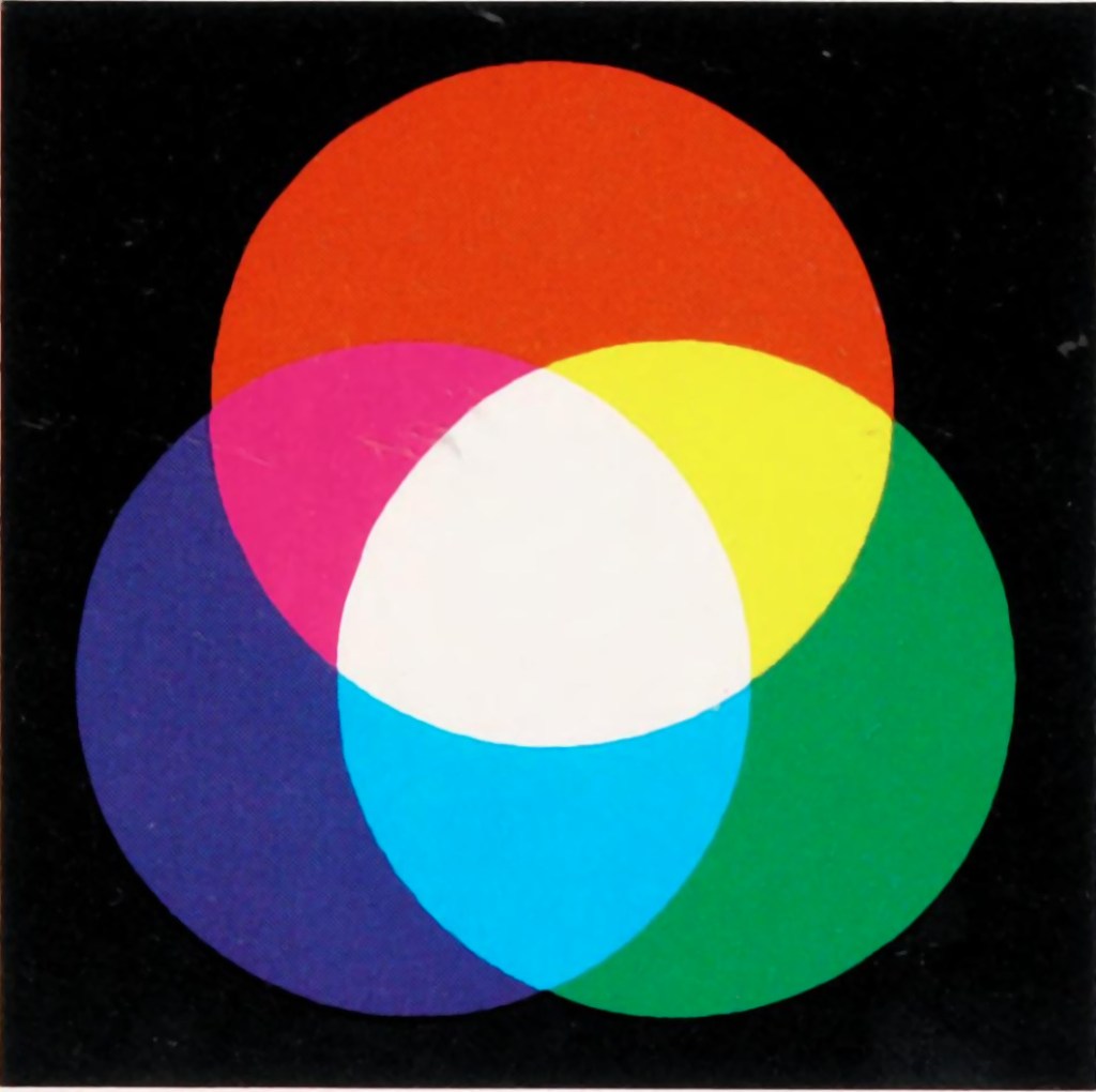
Additive colours are so-called because colours are built by combining wavelengths of light. As more colours are added, the overall colour becomes whiter. Add green and blue together and what you get is a washed out cyan. RGB is an example of an additive colour model. mixing various amounts of red, green, and blue produces the secondary colours: yellow, cyan, and magenta. Additive colour models are the norm for most systems of photograph acquisition or viewing.
Additive colour
Subtractive colour
Subtractive colour works the other way, by removing light. When we look at a clementine, what we see is the orange light not absorbed by the clementine, i.e. all other wavelengths are absorbed, except for orange. Or rather the clementine is subtracting the other wavelengths from the visible light, meaning there is only orange left to reflect off. CMYK and RYB (Red-Yellow-Blue) are good examples of subtractive colour models. Subtractive models are for most systems for printed material.
Different colour inks absorb and reflect specific wavelengths. CMYK (0,0,0,0) looks like white (no ink is laid down, so no light is absorbed), whereas (0,0,0,100) looks like black (maximum black is laid down meaning all colours are absorbed). CMYK values range from 0-100%. Below are some examples.
Lenses used on crop-sensor cameras are a little different to those of full-frame cameras. Mostly this has to do with size – because the sensor is smaller, the image circle doesn’t need to be as large, and therefore less glass is needed in their construction. This allows crop-sensor lenses to be more compact, and lighter. The benefit is that for lenses like telephoto, a smaller size lens is required. A 300mm FF equivalent in MFT only needs to be 150mm. But what does focal-length equivalency mean?
Focal-Length Equivalency
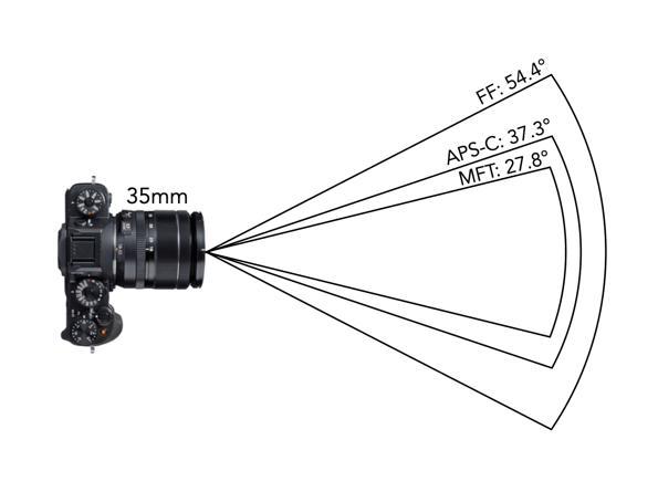
The most visible effect of crop-sensors on lenses is the angle-of-view (AOV), which is essentially where the term crop comes from – the smaller sensor’s AOV is a crop of the full frame. Take a photograph with two cameras: one with a full-frame and another with an APS-C sensor, from the same position using lens with the same focal lengths. The camera with the APS-C sensor will have a more narrowed AOV. For example a 35mm lens on a FF camera has the same focal length as a FF on an MFT or APS-C camera, however the AOV will be different on each. An example of this is shown in Fig.1 for a 35mm lens (showing horizontal AOV).
Fig.1: AOV for 35mm lenses on FF, APS-C, and MFT
Now it should be made clear that none of this affects the focal length of the lens. The focal length of a lens remains the same – regardless of the sensor on the camera. Therefore a 50mm lens in FF, APS-C or MFT will always have a focal length of 50mm. What changes is the AOV of each of the lenses, and consequently the FOV. In order to obtain the same AOV on a cropped-sensor camera, a new lens with the appropriate focal length must be chosen.
Manufacturers of crop-sensors like to use the term “equivalent focal length“. Now this is the focal length AOV as it relates to full-frame. So Olympus says that a MFT lens with a focal length of 17mm has a 34mm FF equivalency. It has an AOV of 65° (diagonal, as per the lens specs), and a horizontal AOV of 54°. Here’s how we calculate those (21.64mm is the diagonal of the MFT sensor, which is 17.3×13mm in size):
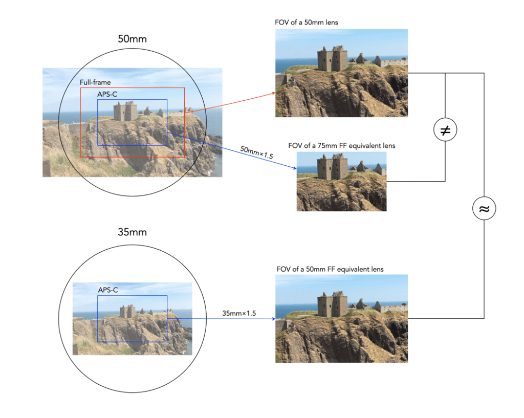
So a lens with a 17mm focal length on a camera with a 2.0× crop factor MFT sensor would give an AOV equivalent of to that of a 34mm lens. An APS-C sensor has a crop factor of ×1.5, so a 26mm lens would be required to give an AOV equivalent of the 34mm FF lens. Figure 2 depicts the differences between 50mm FF and APS-C lenses, and the similarities between a 50mm FF lens and a 35mm APS-C lens (which give approximately the same AOV/FOV).
Fig.2: Example of lens equivalencies: FF vs. APS-C (×1.5)
Interchangeability of Lenses
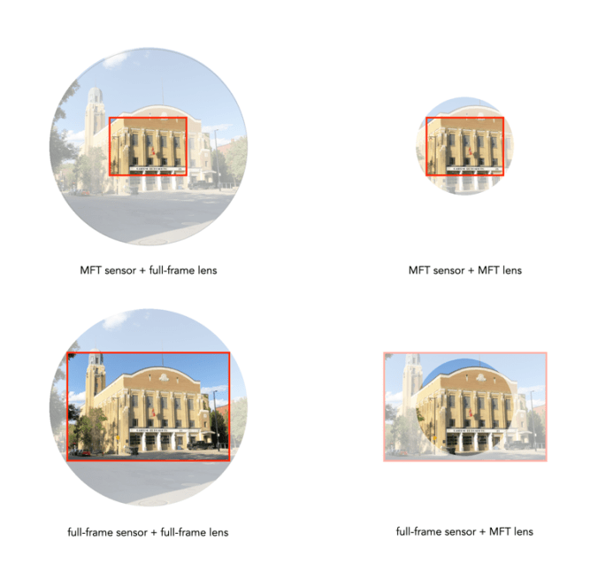
On a side note, FF lenses can be used on crop-sensor cameras because the image circle of the FF lens is larger than the crop sensor. The reverse is however not possible, as a CS lens has a smaller image circle than a FF sensor. The picture below illustrates the various combinations of FF/MFT sensor cameras, and FF/MFT lenses.
Fig.3:The effect of interchanging lenses between FF and crop sensor cameras.
Of course all this is pointless if you don’t care about comparing your crop-sensor camera to a full-frame camera.
NOTE: I tend to use horizontal AOV rather than the manufacturers more typical diagonal AOV. It makes more sense because I am generally viewing a scene in a horizontal context.
DIP is the Digital Image Processing system. Once the ADC has performed its conversion, each of the values from the photosite has been converted from a voltage to a binary number representing some value in its bit depth. So basically you have a matrix of integers representing each of the original photosites. The problem is that this is essentially a matrix of grayscale values, with each element of the matrix representing with a Red, Green of Blue pixel (basically a RAW image). If a RAW image is required, then no further processing is performed, the RAW image and its associated metadata are saved in a RAW image file format. However to obtain a colour RGB image and store it as a JPEG, further processing must be performed.
First it is necessary to perform a task called demosaicing (or demosaiking, or debayering). Demosaicing separates the red, green, and blue elements of the Bayer image into three distinct R, G, and B components. Note a colouring filtering mechanism other than Bayer may be used. The problem is that each of these layers is sparse – the green layer contains 50% green pixels, and the remainder are empty. The red and blue layers only contain 25% of red and blue pixels respectively. Values for the empty pixels are then determined using some form of interpolation algorithm. The result is an RGB image containing three layers representing red, green and blue components for each pixel in the image.
The DIP process
Next any processing related to settings in the camera are performed. For example, the Ricoh GR III has two options for noise reduction: Slow Shutter Speed NR, and High-ISO Noise Reduction. In a typical digital camera there are image processing settings such as grain effect, sharpness, noise reduction, white balance etc. (which don’t affect RAW photos). Some manufacturers also add additional effects such as art effect filters, and film simulations, which are all done within the DIP processor. Finally the RGB image image is processed to allow it to be stored as a JPEG. Some level of compression is applied, and metadata is associated with the image. The JPEG is then stored on the memory card.
Terms used to describe colours are often confusing. If a colour space is a subset of a colour model, then what is a colour gamut? Is it the same as a colour space? How does it differ from a colour profile? In reality there is often very little difference between the terms. For example, depending on where you read it sRGB can be used to describe a colour space, a colour gamut, or a colour profile. Confused? Probably.
Colour gamuts
A gamut is a range or spectrum of some entity, for example “the complete gamut of human emotions“. A colourgamut describes a subset of colours within the entire spectrum of colours that are identifiable by the human eye, i.e. the visible colour spectrum. More specifically a gamut is the range of colours a colour space can represent.
While the range of colour imaging devices is very broad, e.g. digital cameras, scanners, monitors, printers, the range of colours they produce can vary considerably. Colour gamuts are designed to reconcile colours that can be used in common between devices. The term colour gamut is usually used in association with electronic devices, i.e. the devices range of reproducible colours, or the range of different colours that can be interpreted by a colour model. A colour gamut can therefore be used to express the difference between various colour spaces, and to illustrate the extent of coverage of a colour space.
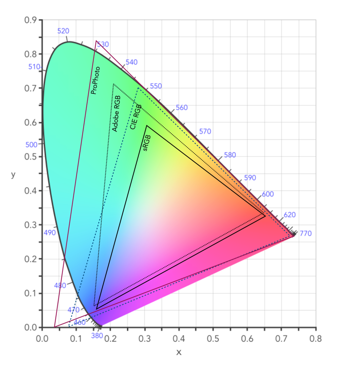
Fig.1: CIE XYZ 2D Chromaticity Diagram depicting various colour spaces as gamuts
The colour gamut of a device is sometimes visualized as a volume of colours, typically in CIELab or CIELuv colour spaces, or as a project in the CIEXYZ colour space producing a 2D xy chromaticity diagram (CD). particularly the luminance of the primary colours. Typically a colour space specifies three (x,y) coordinates to define the three primary colours it uses. The triangle formed by the three coordinates encloses the gamut of colours that the device can reproduce. The table below shows the RGB coordinates for various colour spaces in the CIE chromaticity diagram, shown on the 2D diagram in Figure 1.
Name
R(x)
R(y)
G(x)
G(y)
B(x)
B(y)
%CIE
sRGB
0.64
0.33
0.3
0.6
0.15
0.06
35
Adobe RGb
0.64
0.33
0.21
0.71
0.15
0.06
50
ProPhoto
0.7347
0.2653
0.1596
0.8404
0.0366
0.0001
91
Apple RGB
0.6250
0.34
0.28
0.5950
0.1550
0.07
33.5
NTSC RGB
0.67
0.33
0.21
0.71
0.14
0.08
54
CIE RGB
0.7346
0.2665
0.2811
0.7077
0.1706
0.0059
Note that colour gamuts are 3D which is more informative than the 2D CD – it captures the nuances of the colour space, particularly the luminance of the primary colours. However the problem with 3D is that it is not easy to plot, and hence the reason a 2D representation is often used (the missing dimension is brightness).
Two of the most common gamuts in the visual industry are sRGB, and Adobe RGB (which are also colour spaces). Each of these gamuts references a different range of colours, suited to particular applications and devices. sRGB is perhaps the most common gamut used in modern electronic devices. It is gamut that covers a good range of colours for average viewing needs, so much so that it is the default standard for the web, and most images taken using digital cameras. The largest RGB working space, ProPhoto is an RGB color space developed by Kodak, and encompasses 90% of the possible colours in the CIE XYZ chromaticity diagram.
Gamut mapping is the conversion of one devices colour space to another. For example the case where an image stored as sRGB is to be reproduced on a print medium with a CMYK colour space. The objective of a gamut mapping algorithm is to translate colours in the input space to achievable colours in the output space. The gamut of an output device depends on its technology. For example, colour monitors are not always capable of displaying all colours associated with sRGB.
Colour profiles
On many systems the colour gamut is described as a colour profile, and more specifically is associated with an ICC Color Profile, which is a standardized system put in place by the international colour consortium. Such profiles help convert the colours in the designated colour space associated with an image to the device. For example the standard profile on Apple laptops is “Color LCD”.Some of the most common RGB ICC profiles are sRGB (sRGB IEC61966-2.1).
The inner workings of a camera are much more complex than most people care to know about, but everyone should have a basic understanding of how digital photographs are created.
The ADC is the Analog-to-Digital Converter. After the exposure of a picture ends, the electrons captured in each photosite are converted to a voltage. The ADC takes this analog signal as input, and classifies it into a brightness level represented by a binary number. The output from the ADC is sometimes called an ADU, or Analog-to-Digital Unit, which is a dimensionless unit of measure. The darker regions of a photographed scene will correspond to a low count of electrons, and consequently a low ADU value, while brighter regions correspond to higher ADU values.
Fig. 1: The ADC process
The value output by the ADC is limited by its resolution (or bit-depth). This is defined as the smallest incremental voltage that can be recognized by the ADC. It is usually expressed as the number of bits output by the ADC. For example a full-frame sensor with a resolution of 14 bits can convert a given analog signal to one of 214 distinct values. This means it has a tonal range of 16384 values, from 0 to 16,383 (214-1). An output value is computed based on the following formula:
ADU = (AVM / SV) × 2R
where AVM is the measured analog voltage from the photosite, SV is the system voltage, and R is the resolution of the ADC in bits. For example, for an ADC with a resolution of 8 bits, if AVM=2.7, SV=5.0, and 28, then ADU=138.
Resolution (bits)
Digitizing steps
Digital values
8
256
0..255
10
1024
0.1023
12
4096
0..4095
14
16384
0..16383
16
65536
0..65535
Dynamic ranges of ADC resolution
The process is roughly illustrated in Figure 1. using a simple 3-bit, system with 23 values, 0 to 7. Note that because discrete numbers are being used to count and sample the analog signal, a stepped function is used instead of a continuous one. The deviations the stepped line makes from the linear line at each measurement is the quantizationerror. The process of converting from analog to digital is of course subject to some errors.
Now it’s starting to get more complicated. There are other things involved, like gain, which is the ratio applied while converting the analog voltage signal to bits. Then there is the least significant bit, which is the smallest change in signal that can be detected.
Some sensors sizes are listed as some form of inch, for example a sensor size of 1″ or 2/3”. The diagonal size of this sensor is actually only 0.43” (11mm). Cameras sensors of the “inch” type do not signify the actual diagonal size of the sensor. These sizes are actually based on old video cameras tubes where the inch measurement referred to the out diameter of the video tube.
The world use to use vacuum tubes for a lot of things, i.e. far beyond just the early computers. Video cameras like those used on NASA’s unmanned deep space probes like Mariner used vacuum tubes as their image sensors. These were known as vidicon tubes, basically a video camera tube design in which the target material is a photoconductor. There were a number of branded versions, e.g. Plumicon (Philips), Trinicon (Sony).
A sample of the 1″ vidicon tube, and its active area.
These video tubes were described using the outside diameter of the overall glass tube, and always expressed in inches. This differed from the area of the actual imaging sensor, which was typically two-thirds of the size. For example, a 1″ sized tube typically had a picture area of about 2/3″ on the diagonal, or roughly 16mm. For example, Toshiba produced Vidicon tubes in sizes of 2/3″, 1″, 1.2″ and 1.5″.
These vacuum tube based sensors are long gone, yet some manufacturers still use this deception to make tiny sensors seem larger than they are.
Image sensor
Image sensor size
Diagonal
Surface Area
1″
13.2×8.8mm
15.86mm
116.16mm2
2/3″
8.8×6.6mm
11.00mm
58.08mm2
1/1.8”
7.11×5.33mm
8.89mm
37.90mm2
1/3”
4.8×3.6mm
6.00mm
17.28mm2
1/3.6″
4.0×3.0mm
5.00mm
12.00mm2
Various weird sensor sizes
For example, a smartphone may have a camera with a sensor size of 1/3.6″. How does it get this? The actual sensor will be approximately 4×3mm in size, with a diagonal of 5mm. This 5mm is multiplied by 3/2 giving 7.5mm (0.295″). 1” sensors are somewhere around 13.2×8.8mm in size with a diagonal of 15.86mm. So 15.86×3/2=23.79mm (0.94″), which is conveniently rounded up to 1″. The phrase “1 inch” makes it seem like the sensor is almost as big as a FF sensor, but in reality they are nowhere near the size.
Various sensors and their fractional “video tube” dimensions.
Supposedly this is also where MFT gets its 4/3 from. The MFT sensor is 17.3×13mm, with a diagonal of 21.64mm. So 21.64×3/2=32.46mm, or 1.28″, roughly equating to 4/3″. Although other stores say 4/3 is all about the aspect ratio of the sensor, 4:3.
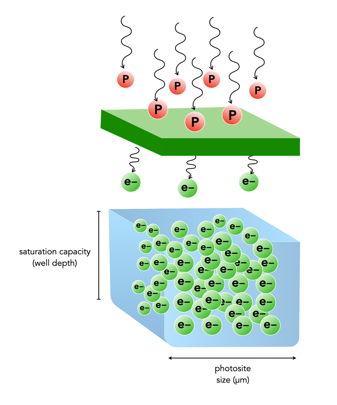
When photons (light) enter a lens of a camera, some of them will pass through all the way to the sensor, and some of those photons will pass through various layers (e.g. filters) and end up in being gathered in the photosite. Each photosite on a sensor has a capacity associated with it. This is normally known as thephotosite well capacity (sometimes called the well depth, or saturation capacity). It is a measure of the amount of light that can be recorded before the photosite becomes saturated (no long able to collect any more photons).
When photons hit the photo-receptive photosite, they are converted to electrons. The more photons that hit a photosite, the more the photosite cavity begins to fill up. After the exposure has ended, the amount of electrons in each photosite is read, and the photosite is cleared to prepare for the next frame. The number of electrons counted determines the intensity value of that pixel in the resulting image. The gathered electrons create a voltage which is an analog signal -the more photons that strike a photosite, the higher the voltage.
More light means a greater response from the photosite. At some point the photosite will not be able to register any more light because it is at capacity. Once a photosite is full, it cannot hold any more electrons, and any further incoming photons are discarded, and lost. This means the photosite has become saturated.
Fig.1: Well-depth illustrated with P representing photons, and e- representing electrons.
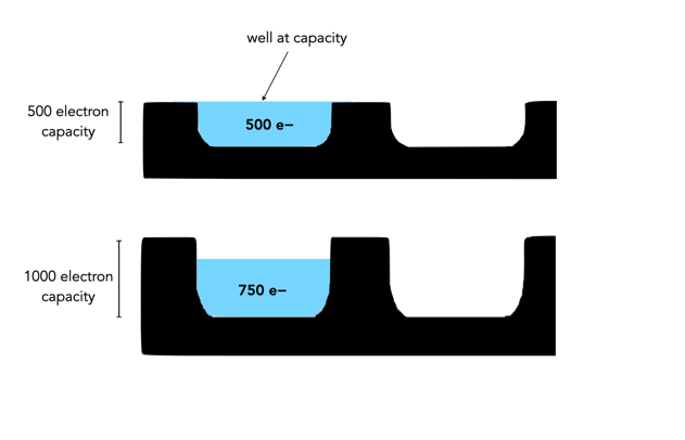
Different sensors can have photosites with different well-depths, which affects how many electrons the photosite can hold. For example consider two photosites from different sensors. One has a well-depth of 1000 electrons, and the other 500 electrons. If everything remains constant from the perspective of camera settings, noise etc., then over an exposure time the photosite with the smaller well-depth will fill to capacity sooner. If over the course of an exposure 750 photons are converted to electrons in each of the photosites, then the photosite with a well-depth of 1000 will be 75% capacity, and the photosite with a well-depth of 500 will become saturated, discarding 250 of the photons (see Figure 2).
Fig.2: Different well capacities exposed to 750 photons
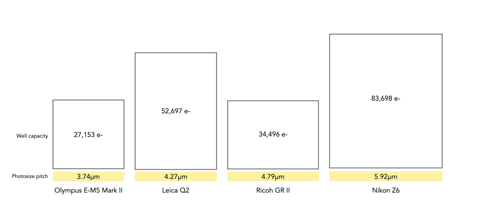
Two photosite cavities with the same well-capacities, but differing size (in μm) will also affect how quickly the cavity fills up with electrons. The larger sized photosite will fill up quicker. Figure 3 shows four differing sensors, each with a different photosite pitch, and well capacity (the area of each box abstractly represents the well capacity of the photosite in relation to the photosite pitch).
Fig.3: Examples of well capacity in various sensors
Of course the reality is that electrons do not need a physical “bin” to be stored in, the photosites are just shown in this manner to illustrate a concept. In fact the concept of well-depth is somewhat ill-termed, as it does not take into account the surface area of the photosite.
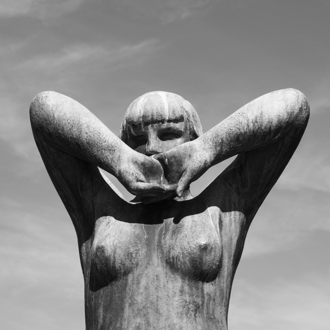
We live in a world where colour surrounds us, so why would anyone want to take an achromatic, black-and-white photograph? What draws us to a B&W photograph? Many modern colour images are brightened to add a sense of the exotic in the same way that B&W invokes an air of nostalgia. B&W does not exaggerate the truth in the same way that colour does. It does sometimes veil the truth, but in many ways it is an equalizer. Colours and the emotions they represent are stripped away, leaving nothing but raw structure. We are then less likely to draw emotions into the interpretation of achromatic photographs. There is a certain rawness to B&W photographs, which cannot be captured by colour.
Every colour image is of course built upon an achromatic image. The tonal attributes provides the structure, the chrominance the aesthetic elements that help us interpret what we see. Black and white photographs offer simplicity. When colour is removed from a photograph, it forces a different perspective of the world. To create a pure achromatic photograph means the photographer has to look beyond the story posed by the chromatic elements of the scene. It forces one to focus on the image. There is no hue, no saturation to distract. The composition of the scene suddenly becomes more important. Both light and the darkness of shadows become more pronounced. The photographic framework of a world without colour forces one to see things differently. Instead of highlighting colour, it helps highlight shape, texture, form and pattern.
Sometimes even converting a colour image to B&W using a filter can make the image content seem more meaningful. Colour casts or odd-ball lighting can often be vanquished if the image is converted. Noise that would appear distracting in a colour image, adds to an image as “grain” in B&W. B&W images will always capture the truth of a subjects structure, but colours are always open to interpretation due to the way individuals perceive colour.
Above is a colour photograph of a bronze sculpture taken at The Vigeland Park in Oslo, a sculpture park displaying the works of Gustav Vigeland. The colour image is interesting, but the viewer is somewhat distracted by the blue sky, and even the patina on the statue. A more interesting take is the achromatic image, obtained via the Instagram Inkwell filter. The loss of colour has helped improve the contrast between the sculpture and its background.
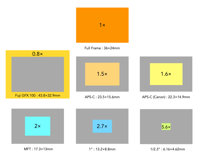
The crop factor of a sensor is the ratio of one camera’s sensor size in relation to another camera’s sensor of a different size. The term is most commonly used to represent the ratio between a 35mm full-frame sensor and a crop sensor. The term was coined to help photographers understand how existing lenses would perform on new digital cameras which had sensors smaller than the 35mm film format.
How to calculate crop factors?
It is easy to calculate a crop factor using the size of a crop-sensor in relation to a full-frame sensor. This is usually determined by comparing diagonals, i.e. full-frame sensor diagonal/cropped sensor diagonal. The diagonals can be calculated using Pythagorean Theorem. Calculate the diagonal of the crop-sensor, and divide this into the diagonal of a full-frame sensor, which is 43.27mm.
Here is an example of deriving the crop factor for a MFT sensor (17.3×13mm):
The diagonal of a full-frame sensor is √(36²+24²) = 43.27mm
The diagonal of the MFT sensor is √(17.3²+13²) = 21.64mm
The crop factor is 43.27/21.64 = 2.0
This means a scene photographed with a MFT sensor will be smaller by a factor or 2 than a FF sensor, i.e. it will have half the physical size in dimensions.
Common crop factors
Type
Crop factor
1/2.3″
5.6
1″
2.7
MFT
2.0
APS-C (Canon)
1.6
APS-C (Fujifilm Nikon, Ricoh, Sony, Pentax)
1.5
APS-H (defunct)
1.35
35mm full frame
1.0
Medium format (Fuji GFX)
0.8
Below is a visual depiction of these crop sensors compared to the 1× of the full-frame sensor.
The various crop-factors per crop-sensor.
How are crop factors used?
The term crop factor is often called the focal length multiplier. That is because it is often used to calculate the “full-frame equivalent” focal length of a lens on a camera with a cropped sensor. For example, a MFT sensor has a crop factor of 2.0. So taking a MFT 25mm lens, and multiplying it by 2.0 gives 50mm. This means that a 25mm lens on a MFT camera would behave more like a 50mm lens on a FF camera, in terms of AOV, and FOV. If a 50mm mounted on a full-frame camera is placed next to a 25mm mounted on a MFT camera, and both cameras were the same distance from the subject, they would yield photographs with similar FOVs. They would not be identical of course, because they have different focal lengths which modifies characteristics such as perspective and depth-of-field.
Things to remember
The crop-factor is a value which relates the size of a crop-sensor to a full-frame sensor.
The crop-factor does not affect the focal length of a lens.
The crop-factor does not affect the aperture of a lens.
Before the advent of digital cameras, the standard reference format for photography was 35mm film, with frames 36×24mm in size. Everything in analog photography had the same frame of reference (well except for medium format, but let’s ignore that). In the early development of digital sensors, there were cost and technological issues with developing a sensor the same size as 35mm film. The first commercially available dSLR, the Nikon QV-1000C, released in 1988, had a ⅔” sensor with a crop-factor of 4. The first full-frame dSLR would not appear until 2002, the Contax N Digital, sporting 6 megapixels.
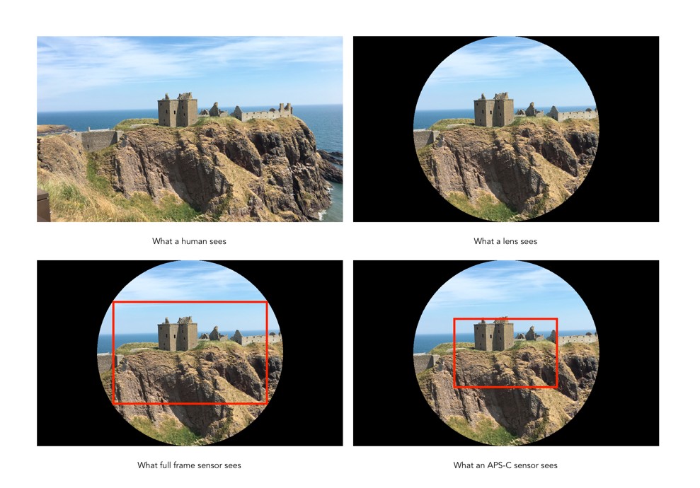
Using a camera with a sensor smaller presented one significant problem – the field of view of images captured using these sensors was narrower than the reference 35mm standard. When camera manufacturers started creating sensors smaller than 36×24mm, they had to create a term which described them in relation to a 35mm film-frame (full-frame). For that reason the term cropsensor is used to describe a sensor that is some percentage smaller than a full-frame sensor (sometimes the term cropped is used interchangeably). The picture a crop sensor creates is “cropped” in relation to the picture created with a full-frame sensor (using the lenses with the same focal length). The sensor does not actually cut anything, it’s just that parts of the image are simply ignored. To illustrate what happens in a full-frame versus a cropped sensor, consider Fig.1.
Fig.1: A visual depiction of full-frame versus crop sensor in relation to the 35mm image circle.
Lenses project a circular image, the “image circle”, but a sensor only records a rectangular portion of the scene. A full-frame sensor, like the one from the Leica SL2 captures a large portion of the 35mm lens circle, whereas the Micro-Four-Thirds cropped sensor of the Olympus OM-D E-M1, only captures the central portion of the lens – the rest of the image falls outside the scope of the sensor (the FF sensor is shown as a dashed box). While crop-sensor lenses are smaller than those of full-frame cameras, there are limits to reducing their size from the perspective of optics, and light capture. Fig.2 shows another perspective on crop sensors based on a real scene, comparing a full-frame sensor to an APS-C sensor (assuming the same “size” lenses, say 50mm).
Fig.2: Viewing full-frame versus crop (APS-C)
The benefits of crop-sensors
Crop-sensors are smaller than full-frame sensors, therefore the cameras are generally smaller. This means cameras are generally smaller in dimensions and weigh less.
The cost of crop-sensor cameras, and the cost of their lenses is generally lower than FF.
A smaller size of lens is required. For example, a MFT camera only requires a 150mm lens to achieve the equivalent of a 300mm FF lens, in terms of field-of-view.
The limitations of crop-sensors
Lenses on a crop-sensor camera with the same focal-length as those on a full-frame camera will generally have a smaller AOV. For example a FF 50mm lens will have an AOV=39.6°, while a APS-C 50mm lens would have an AOV=26.6°. To get a similar AOV on the cropped sensor APS-C, a 33mm equivalent lens would have to be used.
A cropped sensor captures less of the lens image circle than a full-frame.
A cropped sensor captures less light than a full-frame (which has larger photosites which are more sensitive to light).
Common crop-sensors
A list of the most common crop-sensor sizes currently used in digital cameras, as well as the average sensor sizes (sensors from different manufacturers can differ by as much as 0.5mm in size), and example cameras is summarized in Table 1. A complete list of sensor sizes can be found here. Smartphones are in a league of their own, and usually have small sensors of the type 1/n”. For example the Apple iPhone 12 Pro max has 4 cameras – the tele camera uses a 1/3.4″ (4.23×3.17mm) sensor, and the tele camera a 1/3.6″ sensor (4×3mm).
Type
Example Cameras
1/2.3″
6.16×4.62mm
Sony HX99, Panasonic Lumix DC-ZS80, Nikon Coolpix P950
1″
13.2×8.8mm
Canon Powershot G7X M3, Sony X100 VII
MFT / m43
17.3×13mm
Panasonic Lumix DC-G95, Olympus OM-D E-M1 Mark III
APS-C (Canon)
23.3×14.9mm
Canon EOS M50 Mark II
APS-C
23.5×15.6mm
Ricoh GRIII, Fuji X-E3, Sony α6600, Sigma sd Quattro
35mm Full Frame
36×24mm
Sigma fpL, Canon EOS R5, Sony α, Leica SL2-S, Nikon Z6II
Medium format
44×33mm
Fuji GFX 100
Table 1: Crop sensor sizes.
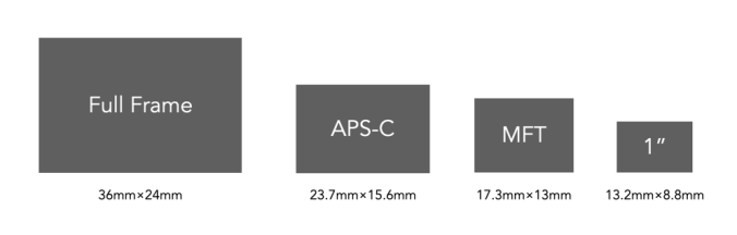
Figure 3 shows the relative sizes of three of the more common crop sensors: APS-C (Advanced Photo System type-C), MFT (Micro-Four-Thirds), and 1″, as compared to a full-frame sensor. The APS-C sensor size is modelled on the Advantix film developed by Kodak, where the Classic image format had a size of 25.1×16.7mm.
Fig.3: Examples of crop-sensors versus a full-frame sensor.
Defunct crop-sensors
Below is a list of sensors which are basically defunct, usually because they are not currently being used in any new cameras.