Converting colour images to grayscale

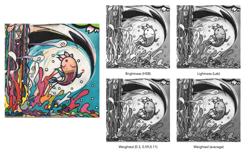
Digital cameras often provide one or more “monochrome” filters, essentially converting the colour image to grayscale (and perhaps adding some form of contrast etc.). How is this done? There are a number of ways, and each will produce a slightly different grayscale image.

All photographs are simulacra, imitations of a reality that is captured by a camera’s film or sensor, and converted to a physical representation. Take a colour photograph, and in most cases there will be some likeness between the colours shown in the picture, and the colours which occur in real life. This may not be perfect, because it is almost impossible to 100% accurately reproduce the colours of real life. Part of this has to do with each person’s intrinsic human visual system, and how it reproduces the colour in a scene. Another part has to do with the type of film/sensor used to acquire the image in the first place. But greens are green, and blues are blue.

Black-and-white images are in a realm of their own, because humans don’t visualize in achromatic terms. So what is a true grayscale equivalent of a colour image? The truth is there is no one single rendition. Though the term B&W derives from the world of achromatic films, even there there is no gold standard. Different films, and different cameras will present the same reality in different ways. There are various ways of acquiring a B&W picture. In an analog world there is film. In a digital world, one can choose a B&W film-simulation from a cameras repertoire of choices, or covert a colour image to B&W. No two cameras necessarily produce the same B&W image.

The conversion of an RGB colour image to a grayscale image involves computing the equivalent gray (or luminance) value Y, for each RGB pixel. There are many ways of converting a colour image to grayscale, and all will produce slightly different results.

  • Convert the colour image to the Lab colour space, and extract the Luminance channel.
  • Extract one of the RGB channels. The one closest is the Green channel.
  • Combine all three channels of the RGB colour space, using a particular weighted formula.
  • Convert the colour image to a colour space such as HSV or HSB, and extract the value or brightness components.
Examples of grayscale images produced using various methods – they may all seem the same, but there are actually subtle differences.

The lightness method

This averages the most prominent and least prominent colours.

Y = (max(R, G, B) + ,min(R, G, B)) / 2

The average method

The easiest way of calculating Y is by averaging the R, G, and B components.

Y = (R + G + B) / 3

Since we perceive red and green substantially brighter than blue, the resulting grayscale image will appear too dark in the red and green regions, and too light in the blue regions. A better approach is using a weighted sum of the colour components.

The weighted method

The weighted method weighs the red, green and blue according to their wavelengths. The weights most commonly used were created for encoding colour NTSC signals for analog television using the YUV colour model. The YUV color model represents the human perception of colour more closely than the standard RGB model used in computer graphics hardware. The Y component of the model provides a grayscale image:

Y = 0.299R + 0.587G + 0.114B

It is the same formula used in the conversion of RGB to YIQ, and YCbCr. According to this, red contributes approximately 30%, green 59% and blue 11%. Another common techniques is to converting RGB to a form of luminance using an equation like Rec 709 (ITU-BT.709), which is used on contemporary monitors.

Y = 0.2126R + 0.7152G + 0.0722B 

Note that while it may seem strange to use encodings developed for TV signals, they are optimized for linear RGB values. In some situations however, such as sRGB, the components are nonlinear.

Colour space components

Instead of using a weighted sum, it is also possible to use the “intensity” component of an alternate colour space, such as the value from HSV, brightness from HSB, or Luminance from the Lab colour space. This again involves converting from RGB to another colour space. This is the process most commonly used when there is some form of manipulation to be performed on a colour image via its grayscale component, e.g. luminance stretching.

Huelessness and desaturation ≠ gray

An RGB image is hueless, or gray, when the RGB components of each pixel are the same, i.e. R=G=B. Technically, rather than a grayscale image, this is a hueless colour image.

One of the simplest ways of removing colour from an image is desaturation. This effectively means that a colour image is converted to a colour space such as HSB (Hue-Saturation-Brightness), where the saturation value is effectively set to zero for all pixels. This pushes the hues towards gray. Setting it to zero is the similar to extracting the brightness component of the image. In many image manipulation apps, desaturation creates an image that appears to be grayscale, but it is not (it is still stored as an RGB image with R=G=B).


Ultimately the particular monochrome filter used by a camera strongly depends on the colour being absorbed by the photosites, because they do not work in monochrome space. In addition certain camera simulation recipes for monochrome digital images manipulate the grayscale image produced in some manner, e.g. increase contrast.

What’s with all the 3rd party ultra-wide and fisheye lenses?

Most large camera manufacturers don’t really make a lot of sub 20mm (FF eq.) lenses. Why? Mostly the cost involved, and likely the lack of sales potential – not many people want to spend a lot of money on a lens that provides a circular fisheye image. I mean these are fun lenses to play with, but in reality aren’t really that practical for everyday use. This may be why 3rd party manufacturers have taken up the mantra, producing low-cost, often reasonable quality sub-20mm lenses. Let’s look at some for Fuji-X.

Let’s divide this into two APS-C categories, the 9-13mm ultra-wide group, and the fisheye group <=8mm. Fisheye lenses can be further categorized into circular and full-frame fisheyes. With regard to focusing MF=manual, AF=auto. Angle-of-view is shown in degrees on the diagonal.

Fisheye lenses: 4-8mm (6-12mm FF)

7artisans Photoelectric 4mm f/2.8 Circular Fisheye (225°) MF US$149
Venus Optics Laowa 4mm f/2.8 Circular Fisheye (210°) MF US$199
Meike MK-6.5mm f/2 Circular Fisheye (190°) MF US$130
7artisans Photoelectric 7.5mm f/2.8 II Fisheye (190°) MF US$139
Pergear 7.5mm f/2.8 (179°) MF US$130
TTArtisan 7.5mm f/2 (190°) MF US$149
Meike 7.5mm f/2.8 Fisheye (180°) MF US$165
Tokina SZ 8mm f/2.8 (180°) MF US$299
Samyang 8mm f/2.8 Fisheye II (180°) MF US$299

Ultra-wide lenses: 9-12mm (13.5-18mm FF)

Venus Optics Laowa 9mm f/2.8 Zero-D (119°) MF US$399
Venus Optics Laowa 10mm f/4 Cookie (109°) MF US$299
Meike 10mm f/2 (107°) MF US$449
ZEISS Touit 12mm f/2.8 (99°) AF US$999
Samyang 12mm f/2.0 NCS CS (99°) MF US$399
7artisans Photoelectric 12mm f/2.8 (102°) MF US$149
Meike MK-12mm f/2.8 (99°) MF US$170
Pergear 12mm f/2 (97°) MF US$160

So which one to choose? It’s really hard to know. It really depends on what you want to do. All these lenses will have some sort of distortion, with the notable exception being the Laowa 9mm, which is described as “Zero-D”. The circular fisheye lenses are nice from an artistic point-of-view, but don’t have that many practical applications (well they are actually used in scientific applications such as assessing forest canopy cover).

Why are these lenses so cheap? Firstly nearly all of the inexpensive lenses, bar the Zeiss 12mm, are manual focus, because obviously incorporating auto-focus mechanisms into any lens is expensive. Another reason may be competition, but it may also be the notion that many of these focal lengths are more for use in an artisanal manner. If these lenses become too expensive, they push themselves out of the market. But inexpensive doesn’t mean a cheap lens. The Laowa 9mm has 15 elements in 10 groups, likely needed to reduce the lenses distortion – so it doesn’t lack good design. Is the Laowa glass inferior to that of Fuji? Possibly, but it’s impossible to tell.

Should you buy an ultra-wide, diagonal fisheye, or even a circular fisheye lens? Well, for the cost involved many of these lenses certainly won’t break the bank, and if you are interested in exploring some artistic photography then it may be a good fit. Which one? Well that’s a bit of a conundrum. Of the six 7.5-8mm lenses, it’s hard to know which is really the best. I would suggest checking out some online reviews, and see what people think of the various lenses.

Why 24-26 megapixels is just about right

When cameras were analog, people cared about resolving power – but of film. Nobody purchased a camera based on resolution because that was contained in the film (and different films have different resolutions). So you purchased a new camera only when you wanted to upgrade features. Analog cameras focused on the tools needed to capture an optimal scene on film. Digital cameras on the other hand focus on megapixels, and the technology to capture photons with photosites, and convert these to pixels. So megapixels are often the name of the game – the first criteria cited when speculation of a new camera arises.

Since the inception of digital sensors, the number of photosites crammed onto various sensor sizes has steadily increased (while at the same time the size of those photosites has decreased). Yet we are now reaching what some could argue is a megapixel balance-point, where the benefits of a jump in megapixels may no longer be that obvious. Is 40 megapixels inherently better than 24? Sure a 40MP image has more pixels, 1.7 times more pixels. But we have to question at what point is there too many pixels? At what point does the pendulum start to swing towards overkill? Is 24MP just about right?

First let’s consider what is lost with more pixels. More pixels means more photosites on a sensor. Cramming more photosites on a sensor will invariably result in smaller photosites (assuming the sensor dimensions do not change). Small photosites mean less light. That’s why 24MB is different on each of MFT, APS-C and full-frame sensors – more space means larger photosites, and better ability in situations such as low-light. Even with computational processing, smaller photosites still suffer from things like increased noise. The larger the sensor, the larger the images produced by the camera, and the greater the post-processing time. There are pros and cons to everything.

Fig.1: Fig: Compare a 24 megapixel image against devices that can view it.

There is also something lost from the perspective of aesthetics. Pictures should not be singularly about resolution, and sharp content. The more pixels you add to an image, there has to be come sort of impact on the aesthetics of an image. Perhaps a sense of hyper-realism? Images that seem excessively digital? Sure some people will like the the highly digital look, with uber saturated colour, and sharp detail. But the downside is that these images tend to lack something from an aesthetic appeal.

Many photographers who long for more resolution are professionals. People who may crop their images, or work on images such as architectural shots or complex landscapes that may require more resolution. Most people however don’t crop their images, and few people make poster-sized prints, so there is little or no need for more resolution. For people that just use photos in a digital context, there is little or no gain. The largest monitor resolution available is 8K, i.e. 7680×4320 pixels, or roughly 33MP, so a 40MP image wouldn’t even display to full resolution (but a 24MP image would). This is aptly illustrated in Figure 1.

Many high-resolution photographs live digitally, and the resolution plays little or no role in how the image is perceived. 24MP is more than sufficient to produce a 24×36 inch print, because nobody needs to pixel-peep a poster. A 24×36” poster has a minimum viewing distance of 65 inches – which at 150dpi, would require a 20MP image.

The overall verdict? Few people need 40MP, and fewer still will need 100MP. It may be fun to look at a 50MP image, but in all practical sense it’s not much better than a 24MP. Resolutions of 24-26MP (still) provide exceptional resolution for many photographic needs. It’s great for magazine spreads (max 300dpi), and fine art prints. So unless you are printing huge posters, it is a perfectly fine resolution for a camera sensor.

Vintage digital – the first full-frame DSLRs

The late 1990s saw a plethora of digital cameras evolve. Some were collaborations between various manufacturers such as Nikon-Fujifilm. But most of these cameras had sensor sizes which were smaller than that of a standard film camera, e.g. APS-C. The first true full-frame cameras appeared in the period 2000-2002.

The first full-frame SLR of note was the Contax N Digital, a 6MP SLR produced by Contax in Japan. Although announced in late 2000, it didn’t actually appear until spring 2002. The sensor was a Philips FTF3020-C, and was only in production for a year before it was withdrawn from the market. Pentax also announced a full-frame camera (using the same sensor as the Contax N), the MZ-D in September 2000, but by October of the following year, the camera had been cancelled. The next full-frame was the Canon EOS-1Ds, which appeared September 2002. It was a monumental step forward, having a full-frame sensor that was 11.1 megapixels. In reality Canon dominated the full-frame market for quite a few years.

Nikon, who stayed in the APS-C for many year was relatively late to the game, not introducing a full-frame until 2007. The Nikon D3 had a modest 12.1MP sensor, but this is because Nikon opted for a low-resolution, high sensitivity sensor. Many lauded the camera for its high ISO noise control, with Popular Photography saying the D3 “will bestow an unheard of flexibility to low-light shooters, or give sports photographers the ability to crank up the shutter speed without adding flash.” To compare, the Canon 2007 equivalent was the Canon EOS-1Ds Mark III, sporting a 21.1MP sensor.

How do these stack up against a modern full-frame? If we compare the Canon 1Ds against a Canon R5C on certain charcteristics:

Canon 1Ds (2002)Canon R5 C (2022)
megapixels1145
ISO100-1250100-51200
video8K
weight1585g770g
number of focus points451053
number of shots per battery600220-320

These early full-frame DSLR’s were certainly beasts from the perspective of weight, and even megapixels, but to be honest 11MP still stacks up today for certain applications.

Further reading:

When more is not always better – the deception of megapixels

I have never liked how companies advertise cameras using megapixels. Mostly because it is quite deceptive, and prompts people to mistakenly believe that more megapixels is better – which isn’t always the case. But the unassuming amateur photographer will assume that 26MP is better than 16MP, and 40MP is better than 26MP. From a purely numeric viewpoint, 40MP is better than 26MP – 40,000,000 pixels outshines 26,000,000 pixels. It’s hard to dispute raw numbers. But pure numbers don’t tell the full story. There are two numeric criteria to consider when considering how many pixels an image has: (i) the aggregate number of pixels in the image, and (ii) the image’s linear dimensions.

Before we look at this further, I just want to clarify one thing. A sensor contains photosites, which are not the same as pixels. Photosites capture light photons, which are then processed in various ways to produce an image containing pixels. So a 24MP sensor will contain 24 million photosites, and the image produced by a camera containing this sensor contains 24 million pixels. A camera has photosites, an image has pixels. Camera manufacturers use the term megapixel likely to make things simpler, besides which megaphotosite sounds more like some kind of prehistoric animal. For simplicities sake, we will use photosite when referring to a sensor, and pixel when referring to an image.

Aggregate pixels versus linear dimensions
Fig.1: Aggregate pixels versus linear dimensions

Every sensor is made up of P photosites arranged in a rectangular shape with a number of rows (r) and a number of columns (c), such that P = r×c. Typically the rectangle shape of the sensor forms an aspect ratio of 3:2 (FF, APS-C), or 4:3 (MFT). The values of r and c are the linear dimensions, which basically represent the resolution of the image in each dimension, i.e. the vertical resolution will be r, the horizontal resolution will be c. For example in a 24MP, 3:2 ratio sensor, r=4000, c=6000. The image aggregate is the number of megapixels associated with the sensor. So r×c = 24,000,000 = 24MP. This is the number most commonly associated with the resolution of an image produced by a camera. In reality, the number of photosites and the number of pixels are equivalent. Now let’s look at how this affects an image.

Doubling megapixels versus doubling linear dimensions
Fig.2: Doubling megapixels versus doubling linear dimensions

The two numbers offer different perspectives of how many pixels are in an image. For example the difference between a 16MP image and a 24MP image is a 1.5 times increase in aggregate pixels. However due to how these pixels are distributed in the image, it only adds up to a 1.25 times increase in the linear dimensions of the image, i.e. there are only 25% more pixels in the horizontal and vertical dimensions. So while upgrading from 16MP to 24MP does increase the resolution of an image, it only adds a marginal increase from a dimensional perspective. Doubling the linear dimensions of an image would require a sensor with 64 million photosites.

A visual depiction of different full-frame sensor sizes for Fuji sensors
Fig.3: A visual depiction of different full-frame sensor sizes for Fuji sensors

The best way to determine the effect of upsizing megapixels is to visualize the differences. Figure 3 illustrates various sensor sizes against a baseline 16MP – this is based on the actual megapixels found in current Fuji camera sensors. As you can see, from 16MP it makes sense to upgrade to 40MP, from 26MP to 51MP, and 40MP to 102MP. In the end, the number of pixels produced by an camera sensor is deceptive in so much as small changes in aggregate pixels does not automatically culminate in large changes in linear dimensions. More megapixels will always mean more pixels, but not necessarily better pixels.

Where did the term “full-frame” originate?

Why are digital cameras with sensors the same size as 35mm SLR’s, i.e. 36×24mm, called full-frame cameras? This is somewhat of a strange concept considering that unlike film, where the 35mm dominated the SLR genre, digital cameras did not originate with 35mm film-equivalent sized sensors. In fact for many years, until the release of the first digital SLRs, camera sensors were of the sub-35mm or “crop-sensor” type. It was not until spring 2002 the first full-frame digital SLR appeared, the 6MP Contax Digital N. It was followed shortly after by the 11.1MP Canon EOS-1Ds. It wouldn’t be until 2007 that Nikon offered its first full-frame-camera, the D3. In all likelihood, the appearance of a sensor equivalent in size to 35mm film was in part because the industry wished to maintain the existing standard, allowing the use of standard lenses, and the existing 35mm hierarchy.

One of the first occurrences of the term “full-frame” as it related to digital, may have been in the advertising literature for Canon’s EOS-1Ds.

“A full-frame CMOS sensor – manufactured by Canon – with an imaging area of 24 x 36mm, the same dimensions used by full-frame 35mm SLRs. It has 11.1 million effective pixels with a maximum resolution of 4,064 x 2,704 pixels.”

Canon EOS-1Ds User Manual, 2002

By the mid 2000’s digital cameras using “crop-sensors” like APS-C had become standard, but the rise of 35mm DSLRs may have triggered a need to re-align the market place towards the legacy of 35mm film. As most early digital cameras used sensors that were smaller than 36×24mm, the term “full-frame” was likely used to differentiate it from smaller sized sensors. But the term has other connotations.

  • It is used in the context of fish-eye lenses to denote an image which covered the full 35mm film frame, as opposed to fish-eye lenses which just manifested as a circle.
  • It is used to denote the use of the entire film frame. For example when film APS-C appeared in 1996, the cameras were able to take a number of differing formats: C, H, and P. H is considered the “full-frame” format with a 9:16 aspect ratio, while P is the panoramic format (1:3), and C the classic 35mm aspect ratio (2:3).

In any case, the term “full-frame” is intrinsically linked to the format of 35mm film cameras. The question is whether or not this term is even relevant anymore?

Pixel peeping and why you should avoid it

In recent years there has been a lot of of hoopla about this idea of pixel peeping. But what is it? Pixel peeping is essentially magnifying an image until individual pixels are perceivable by the viewer. The concept has been around for many years, but was really restricted to those that post-process their images. In the pre-digital era, the closest photographers would come to pixel peeping was the use of a loupe to view negatives, and slides in greater detail. It is the evolution of digital cameras that spurned the widespread use of pixel peeping.

Fig.1: Peeping at the pixels

For some people, pixel-peeping just offers a vehicle for finding flaws, particularly in lenses. But here’s the thing, there is no such thing as a perfect lens. There will always be flaws. A zoomed in picture will contain noise, and grain, unsharp, and unfocused regions. But sometimes these are only a problem because they are being viewed at 800%. Yes, image quality is important, but if you spend all your time worrying about every single pixel, you will miss the broader context – photography is suppose to be fun.

Pixel-peeping is also limited by the resolution of the sensor, or put another way, some objects won’t look good when viewed at 1:1 at 16MP. They might look better at 24MP, and very good at 96MP, but a picture is the sum of all its pixels. My Ricoh GR III allows 16× zooming when viewing an image. Sometimes I use it just to find out it the detail has enough sharpness in close-up or macro shots. Beyond that I find little use for it. The reality is that in the field, there usually isn’t the time to deep dive into the pixel content of a 24MP image.

Of course apps allow diving down to the level of the individual pixels. There are some circumstances where it is appropriate to look this deep. For example viewing the subtle effects of changing settings such as noise reduction, or sharpening. Or perhaps viewing the effect of using a vintage lens on a digital camera, to check the validity of manual focusing. There are legitimate reasons. Pixel peeping on the whole is really only helpful for people who are developing or finetuning image processing algorithms.

Fig.2: Pixel peeping = meaningless detail

One of the problems with looking at pixels 1:1 is that a 24MP image was never meant to be viewed using the granularity of a pixel. Given the size of the image, and the distance it should be viewed at, micro-issues are all but trivial. The 16MP picture in Figure 2 shows pixel-peeping of one of the ducks under the steam engine. The entire picture has a lot of detail in it, but dig closer, and the detail goes away. That makes complete sense because there are not enough pixels to represent everything in complete detail. Pixel-peeping shows the ducks eye – but it’s not exactly that easy to decipher what it is?

People that pixel-peep are too obsessed with looking at small details, when they should be more concerned with the picture as a whole.

What is an RGB colour image?

Most colour images are stored using a colour model, and RGB is the most commonly used one. Digital cameras typically offer a specific RGB colour space such as sRGB. It is commonly used because it is based on how humans perceive colours, and has a good amount of theory underpinning it. For instance, a camera sensor detects the wavelength of light reflected from an object and differentiates it into the primary colours red, green, and blue.

An RGB image is represented by M×N colour pixels (M = width, N = height). When viewed on a screen, each pixel is displayed as a specific colour. However, deconstructed, an RGB image is actually composed of three layers. These layers, or component images are all M×N pixels in size, and represent the values associated with Red, Green and Blue. An example of an RGB image decoupled into its R-G-B component images is shown in Figure 1. None of the component images contain any colour, and are actually grayscale. An RGB image may then be viewed as a stack of three grayscale images. Corresponding pixels in all three R, G, B images help form the colour that is seen when the image is visualized.

A Decoupled RGB image
Fig.1: A “deconstructed” RGB image

The component images typically have pixels with values in the range 0 to 2B-1, where B is the number of bits of the image. If B=8, the values in each component image would range from 0..255. The number of bits used to represent the pixel values of the component images determines the bit depth of the RGB image. For example if a component image is 8-bit, then the corresponding RGB image would be a 24-bit RGB image (generally the standard). The number of possible colours in an RGB image is then (2B)3, so for B=8, there would be 16,777,216 possible colours.

Coupled together, each RGB pixel is described using a triplet of values, each of which is in the range 0 to 255. It is this triplet value that is interpreted by the output system to produce a colour which is perceived by the human visual system. An example of an RGB pixel’s triplet value, and the associated R-G-B component values is shown in Figure 2. The RGB value visualized as a lime-green colour is composed of the RGB triplet (193, 201, 64), i.e. Red=193, Green=201 and Blue=64.

Fig.2: Component values of an RGB pixel

One way of visualizing the R,G,B, components of an image is by means of a 3D colour cube. An example is shown in Figure 3. The RGB image shown has 310×510, or 158,100 pixels. Next to it is a colour cube with the three axes, R, G, and B, each with a range of values 0-255, producing a cube with 16,777,216 elements. Each of the images 122,113 unique colours is represented as a point in the cube (representing only 0.7% of available colours).

Fig 2 Example of colours in an RGB 3D cube

The caveat of the RGB colour model is that it is not a perceptual one, i.e. chrominance and luminance are not separated from one another, they are coupled together. Note that there are some colour models/space that are decoupled, i.e. they separate luminance information from chrominance information. A good example is HSV (Hue, Saturation, Value).

Demystifying Colour (ix) : CIE chromaticity diagram

Colour can be divided up into luminosity and chromaticity. The CIE XYZ colour space was designed such that Y is a measure of the luminance of a colour. Consider a 3D plane is described by X=Y=Z=1, as shown in Figure 1. A colour point A=(Xa,Ya,Za) is then found by intersecting the line SA (S=starting point, X=Y=Z=0) with the plane formed within the CIE XYZ colour volume. As it is difficult to perceive 3D spaces, most chromaticity diagrams discard luminance and show the maximum extent of the chromaticity of a particular 2D colour space. This is achieved by dropping the Z component, and projecting back onto the XY plane.

Fig.1: CIE XYZ chromaticity diagram derived from CIE XYZ open cone.
Fig.2: RGB colour space mapped onto the chromaticity diagram

This diagram shows all the hues perceivable by the standard observer for various (x, y) pairs, and indicates the spectral wavelengths of the dominant single frequency colours. When Y is plotted against X for spectrum colours, it forms a horseshoe, or shark-fin, shaped diagram commonly referred to as the CIE chromaticity diagram where any (x,y) point defines the hue and saturation of a particular colour.

Fig.3: The CIE Chromaticity Diagram for CIE XYZ

The xy values along the curved boundary of the horseshoe correspond to the “spectrally pure”, fully saturated colours with wavelengths ranging from 360nm (purple) to 780nm (red). The area within this region contains all the colours that can be generated with respect to the primary colours on the boundary. The closer a colour is to the boundary, the more saturated it is, with saturation reducing towards the “neutral point” in the centre of the diagram. The two extremes, violet (360nm) and red (780nm) are connected with an imaginary line. This represents the purple hues (combinations of red and blue) that do not correspond to primary colours. The “neutral point” at the centre of the horseshoe (x=y=0.33) has zero saturation, and is typically marked as D65, and corresponds to a colour temperature of 6500K.

Fig.4: Some characteristics of the CIE Chromaticity Diagram

The basics of the X-Trans sensor filter

Many digital cameras use the Bayer filter as a means of capturing colour information at the photosite level. Bayer filters have colour filters which repeat in 2×2 pattern. Some companies, like Fuji use a different type of filter, in Fuji’s case the X-Trans filter. The X-Trans filter appeared in 2012 with the debut of the Fuji X-Pro1.

The problem with regularly repeating patterns of coloured pixels is that they can result in moiré patterns when the photograph contains fine details. This is normally avoided by adding an optical low-pass filter in front of the sensor. This has the affect of applying a controlled blur on the image, so sharp edges and abrupt colour changes and tonal transitions won’t cause problems. This process makes the moiré patterns disappear, but at the expense of some image sharpness. In many modern cameras the sensor resolution often outstrips the resolving power of lenses, so the lens itself acts as a low-pass filter, and so the LP filter has been dispensed with.

Bayer (left) versus X-Trans colour filter arrays

C-Trans uses a more complex array of colour filters. Rather than the 2×2 RGBG Bayer pattern, the X-Trans colour filter uses a larger 6×6 array, comprised of differing 3×3 patterns. Each pattern has 55% green, 22.5% blue and 22.5% red light sensitive photosite elements. The main reason for this pattern was to eliminate the need for a low-pass filter, because this patterning reduces moiré. This theoretically strikes a balance between the presence of moiré patterns, and image sharpness.

The X-Trans filter provides a for better colour production, boosts sharpness, and reduces colour noise at high ISO. On the other hand, more processing power is needed to process the images. Some people say it even has a more pleasing “film-like” grain.

CharacteristicX-TransBayer
Pattern6×6 allows for more organic colour reproduction.2×2 results in more false-colour artifacts.
MoiréPattern makes images less susceptible to moiré.Bayer filters contribute to moiré.
Optical filterNo low-pass filer = higher resolution.Low-pass filter compromises image sharpness.
ProcessingMore complex to process.Less complex to process.
Pros and Cons between X-Trans and Bayer filters.

Further reading: