When lenses first appeared they had a particular shape, a double convex lens, that was very similar to a certain pulse, namely the lentil. The name lens derived from the Latin name for the plant, lens culinaris.
“LENS (Latin , lens, a small bean or lentil). A lens is a piece of transparent material (usually glass) bounded by curved surfaces (generally spherical, including flat).
An English dictionary of the early 18th century [1] describes a lens as related to optics to be a “small concave or convex glass”. By 1768 [2] it was described as “a glass, spherically convex on both sides”.
The word lentil comes from the Old French lentille, which in turn comes from Latin lenticula. When lenses first appeared, they looked like the lentil seed, and likely due to the fact that technical terms were derived from Greek or Latin, simply named them lens. In German, one term used is Linse, but it is more common to use the term Objektiv. The term Linse is from the Old High German linsa, from a Proto-Indo-European root.
Dictionarium Anglo-Britannicum, John Kersey (1708)
A Dictionary of the English Language, Samuel Johnson (1768)
Why was the 50mm lens considered the “normal” lens used on 35mm cameras? Why not 40mm or 60mm? When Barnack introduced his revolutionary Leica camera, he used a traditional method of selecting the lens – the most commonly used lens has a focal length should be approximately equal to the diagonal of the negative, which is how the 50mm likely evolved. The Leica I came with a fixed 50mm lens, and even when the Leica II appeared in 1932 with interchangeable lenses, the viewfinder was designed to work with 50mm lenses. Zeiss Contax lens brochures from the 1930s mark 50mm lenses as “universal lenses”, “For all-round use and subjects which occur in every-day photography…”. Nikon also made the point that “Nikkor normal lenses cover a picture angle of approximately 45°, corresponding closely to the angle of view of the human eye”.
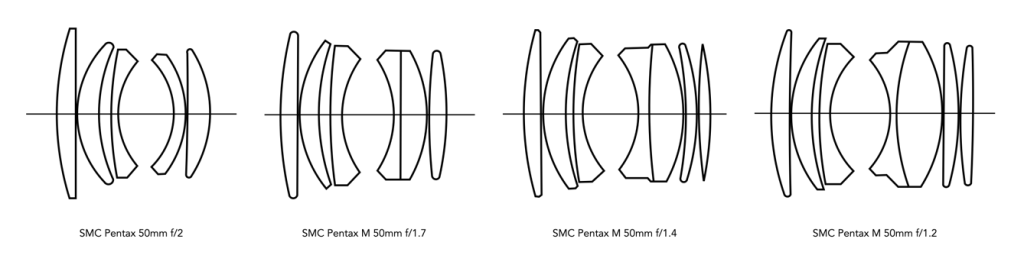
It is then no surprise that 50mm is the most ubiquitous analog lens. By the 1950s, most interchangeable lens cameras came standard with a 50mm lens, ensuring that novice photographers could capture sharp photographs in a variety of conditions without requiring a books worth of knowledge. Nikon in one of their lens brochures suggested “the 50mm focal length has become the standard lens for all around work”. This deep-seeded ideology is probably why 50mm lenses came in so many speeds – the same Nikon brochure provides an f/3.5, f/2, f/1.4, and f/1.1 50mm lenses. Many camera manufacturers followed suit. The late 1970s “standard” line-up for Asahi Pentax included four 50mm lenses (f/1.2, f/1.4, f/1.7, f/2) and a 40mm f/2.8 which they touted as being “extremely versatile”.
Fig.1: How many normal’s is too many normal’s? (Pentax SMC lenses)
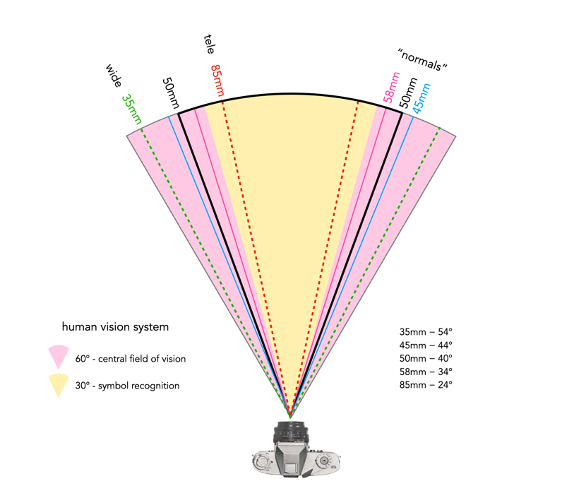
There are a number of arguments that have traditionally been made as to why 50mm is “normal”. The most common argument of course is that the 50mm lens has a diagonal angle-of-view (AOV) of about 45° which approximates the AOV of the human eye. But in reality it makes assumptions about what “normal vision” is , and the ability of a 50mm lens to reproduce it. The idea that 50mm best approximates human vision has more to do with the evolution of lenses than it has to do with any correspondence between the human eye and a lens. There are other arguments, for instance that 50mm reproduces facial proportions, depth and perspective roughly as how our eyes perceive them. Many manufacturers drove this point home by saying 50mm lenses “give pictures of natural, i.e. normal, perspective”.
Fig.2: Angle of views of the human vision system
Firstly we should remember that “normal” human vision is binocular, while camera lenses are not. The eye is also composed of a gel-like material, versus the glass of lens elements. So there are already fundamental structural and functional differences. There is also the matter of AOV. A lens generally has one AOV, whereas the human visual system (HVS) has a series, based on differing abilities to focus – binocular vision is approximately 120° of view, of which only 60° is the central field of vision (the remainder is peripheral vision), and only 30° of that is vision capable of symbol recognition (even less is capable of sharp focusing, perhaps 5°?). Note that I use horizontal AOV in comparisons, because it is easier for people to conceptualize than diagonal AOV.
Fig.3: AOV of various lens focal lengths against the AOV of the human vision system
In reference to Figure 3, for the hard limits, a 67mm lens would likely best approximate the 30° region of the HVS that deals with symbol recognition, whereas a 31mm would best approximate the 60° central field of vision. If we were simply to take the middle ground, at 45°, we get a 43mm lens, which actually matches the diagonal of the 24×36mm frame.
But how closely does the 50mm AOV resembles that of the human visual system (HVS)? In terms of horizontal vision, a 50mm lens has a 40° AOV, so it’s not that far removed from that of the 43mm lens. Part of the problem lies with the fact that it is hard to establish an exact value that represents the “normal viewing angle” of the HVS. This is why other lens fit into this “normal” category – the 40mm (48°), the 45mm (44°), the 55mm (36°) and the 58mm (34°). Herbert Keppler may have put it best in his book The Asahi Pentax Way (1966):
“A normal focal length lens on any camera is considered to be a lens whose focal length closely approximates the diagonal of the picture area produced on the film. With 35mm cameras, this actually works out to be about 43mm, generally considered a little too short to produce the best angle of coverage and most pleasing perspective. Consequently, makers of 35mm cameras have varied their “normal” focal lengths between 50 and 58mm. With early single lens reflexes the longer 58mm length was in general use. However, in recent years there seems to be a trend to slightly shorter focal lengths which produce a greater angle of view. Current Pentax models use both 50 and 55mm focal length lenses.”
In some respects it seems like 50mm was chosen because it is close to what could be perceived as the AOV of the HVS, such that it is, and provided a nice rounded focal length value. By the 1950s, the 50mm had become “the standard” lens, with 35mm and 85mm lenses providing wide and telephoto capabilities respectively (a 35mm lens has an AOV of 54°, and the 85mm lens has an AOV of 24°, and surprisingly, 50mm sits smack dab in the middle of these). Many brochures simply identified it as an “all-round” lens. It is difficult to pinpoint where the reference of 50mm approximating the AOV of the human eye may have first appeared.
With the move to digital, the exact notion of a 50mm “normal” lens has not exactly persevered. This is primarily because the industry has moved away from 36×24mm being the normal film/sensor size, even though we hang onto the idea of 35mm equivalency. While a 50mm lens might be considered “normal” on a full-frame sensor, on an APS-C sensor a “normal” lens would be 35mm, because it is “equivalent” to a 50mm full-frame lens, from the perspective of focal length and more importantly AOV. Note that Zeiss still allude to the fact that the “focal length of the ZEISS Planar T* 1.4/50 is equal to the perspective of the human eye.”
“The world is three-dimensional; a photographic image is two-dimensional. Because of this flatness, the depth of depictive space always always bears a relationship to the picture plane. The picture plane is a field upon which the lens’s image is projected. A photographic image can rest on this picture plane and, at the same time, contain an illusion of deep space.”
“There is no such thing as an instantaneous photograph. All photographs are time exposures, of shorter or longer duration, and each describes a discrete parcel of time. This time is always the present. Uniquely in the history of pictures, a photograph describes only that period of time in which it was made. Photography alludes to the past and the future only in so far as they exist in the present, the past through its surviving relics, the future through prophecy visible in the present.”
So who made f/1.2 lenses? The answer is that most manufacturers had some lenses with this large aperture, usually in the 50-60mm range. Most of these lenses came from Japanese manufacturers, who led the way in fast lenses. The only real exception is the Leitz Wetzlar Noctilux 50mm, and they are expensive, to the point where it is cheaper to buy a new Noctilux-M 50mm f/1.2 ASPH (for US$8k).
These lenses are sorted by focal length and years up to 1985. Up until 1975, there were few if any 50mm f/1.2 lenses for SLR cameras, but there were a range of 55/58mm f/1.2 lenses. Note R indicates a lens for a rangefinder camera.
In the 1940s, a lens speed of f/3.5 was quite normal, an f/2 very fast. The world first f/1.4 lens for a 35mm camera appeared in 1950, when Nikon released the NIKKOR-S 5cm f/1.4. That sparked a series of f/1.4 lenses from most manufacturers. But this wasn’t fast enough. In the world of vintage lenses, f/1.2 lenses are almost the holy grail. Fujinon was the first to introduce an f/1.2 5cm lens in 1954 for rangefinder cameras. Canon introduced a 50mm f/1.2 lens, for the Canon S series in 1956. Many manufacturers followed suit, producing one or more lenses in the decades to come. Japanese camera companies lead the way in super-fast normal lenses. Some milestones:
First f/1.2 for SLR (1962) – Canon Super-Canonmatic R 58mm f/1.2
First f/1.2 55mm lens (1965) – Nikon Nikkor-S Auto 55mm f/1.2
First f/1.2 50mm lens for SLR (1975) – Pentax SMC 50mm f/1.2
Fig.1: The ever increasing complexities of optical elements in lenses with large apertures from f/2 to f/1.2(Asahi Pentax)
Aside from the fact that these f/1.2 lenses represent the pinnacle of wide-open lenses of the period, what makes them so expensive (both then and now)?
Rarity – Although a large number of manufacturers developed f/1.2 lenses, in may cases fewer were manufactured than slower lenses. For example, the Fujinon 5cm f/1.2 lens was made in limited amounts, less than 1000 by all accounts, but because of this ranges from $4000-20000.
Larger glass – As the speed of a lens increased, so too did the size of its optical elements. An f/1.2 lens had much more glass than say an f/2.8, e.g. a 50mm f/2.8 lens would have an effective aperture of 25mm, while an f/1.2 50mm would have one of 41.7mm. This means the optical elements had to be much larger for an f/1.2 lens.
Better glass – Larger optical elements also mean they had to be of a higher quality, with less tolerance for defects such as bubbles. Some optical elements may have been made of rare-earth metals to improve optical qualities, and reduce aberrations.
More optical elements – As lenses got faster, more elements needed to be added to counter optical aberrations.
Inner mechanisms – Larger optical elements meant one of two things for the lens housing (i.e. barrel): (i) make it a lot larger, and therefore increase the size of all the components, or (ii) make it marginally larger, and reduce the size of the mechanisms within the lens, e.g. aperture control, so they become more compact.
Complexmanufacturing – Specialized glass needed new processes to ensure high manufacturing tolerances, e.g. finer levels of polishing.
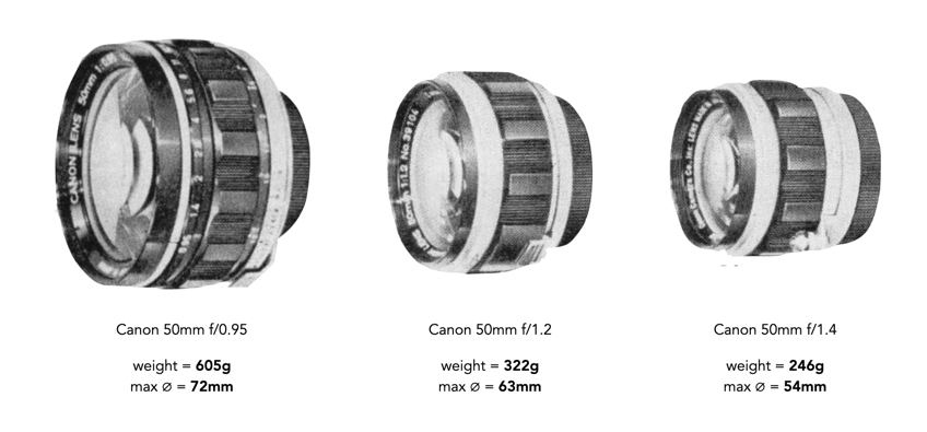
Fig.2: The ever increasing size and weight of lenses with large apertures(the Canon rangefinder series)
All these elements contributed to an increase in the cost of these “revolutionary” lenses. However, although we consider them expensive now, f/1.2 lenses were always expensive. In 1957, the Canon 50mm f/1.2 rangefinder lens sold for US$250, with the Fujinon 50mm f/1.2 at $299.50 [1]. The Canon 50mm f/1.8 on the other hand sold for $125, and a Canon V with a 50mm f/1.8 lens sold for $325. A 1970 Canon price [2] list provides a better perspective, with information for the lenses for the Canon 7/7s rangefinder. The slower 50mm lens sold for $55 (f/2.8), and $120 (f/1.8), while the f/1.4 sold for $160 and the f/1.2 for $220 (the f/0.95 was the most expensive at $320). SLR lenses were cheaper, although Canon did not make a 50mm f/1.2 (until 1980), it did make a 55mm f/1.2, which sold for $165.
Note that $220 in 2022 dollars is $1608. Today, some of these lenses fetch a good price, depending on condition. The Canon 50mm f/1.2 sells for around $400-600 based on condition. The series of f/1.2 lenses made by Tomioka Kogaku circa 1970 regularly sell for between C$800-1700.
The price of nostalgia.
Further reading:
“Photographic Lenses”, Popular Photography 40(4), April, p.168 (1957)
Canon Systems Equipment, Bell & Howell Co. March 1970
“It’s a great temptation, especially here in Japan, where really beautiful precision cameras and lenses ca be had for a fraction of the cost in the United States, to add just one more to an already over-stuffed gadget bag.
Don’t however, be led into the error of thinking that the answer to good pictures is to be found in a complete set of matched lenses. Just the opposite is true, for there is a very definitive correlation between the number of lenses the average photographer carries, and the worth-while pictures he produces. Unfortunately, this varies in inverse order; in other words, the more equipment to worry about, the fewer pictures of merit!
Special demand will require special equipment. For example, any photographer specializing in portraits or stage photography will find the f2 Serenar 85mm indispensable, but neither this or any number of lenses will do more than allow you to take better pictures. In fact, you chances of becoming a great photographer are probably better with only one lens, than with one hundred.”
Horace Bristol, TOKYO on a five day pass; with candid camera (1951).
On the basis of the previous posts, this posts presents a method of generating a digital contact sheet using another ImageMagick command, montage. It can be used for pure images, or as I like to do, create a contact sheet with the images and their intensity histograms. Like many commands there are a myriad of options, but a basic use of montage might be:
This takes all PNG files in the current directory and creates an 8×5 montage (8 columns by 5 rows) with 200×150 thumbnails of the images, and saves the montage in a file named contact.png. This will hold 40 images, and if there are more than this, they spill over into a second image. This is a little bit awkward, so to make things nicer, we can write a script to process the images. Below is a bash shell script called contactsheet.sh :
#!/bin/bash
ls *.png > imglist
read nImgs <<< $(sed -n '$=' imglist)
let nrows=nImgs/8
let lefto=nImgs%8
if [ $lefto -gt 0 ]
then
   let nrows=nrows+1
fi
montage @imglist -geometry 200x150 -tile 8x$nrow $1
rm imglist
Now let’s look through this script based on what each line does.
Line 1 Identifies the script as a bash shell script.
Line 2 uses the ls command to list all the PNG image files in the current directory, and outputs the list to a text file called imglist. The files will be sorted in alphabetical order.
Line 3 counts the number of lines in the file imglist, using the sed (stream editor) command, sed -n '$=' imglist. The number of lines represents the number of PNG files, as there is one filename per line. The number of files calculated is stored in the variable nImgs.
Line 4 calculates the number of rows by dividing nImgs by 8, and stores the value in the variable nrows (assuming we want 8 images across in the montage). This will produce an integer result. For example if the number of images is 41, then 41/8 = 5.
Line 5 calculates the leftover from the division of nImgs by 8, and stores it in the variable lefto. For example 41%8 = 1.
Line 6 questions if the leftover, i.e. the value in lefto, is greater than 0. If it is, it indicates a extra row should be added to the variable nrows (Line 8). This deals with the issue of montage creating an extra image should the number of images go beyond the 8×5 tiles.
Line 10, generates the contact sheet using montage. It uses the list in imglist, and uses the variable nrows to specify the number of rows in the montage, i.e. 8x$nrow. The $1 at the end of the command is the output filename for the montage, which is specified when contactsheet is run, for example (result shown in Fig.1):
./contactsheet.sh photosheet1.png
Line 11 deletes the file containing the list of images.
Fig.1: A sample digital contact sheet using the script.
It may seem quite complicated, but once you get the hang of it, writing these scripts save a lot of time. If you have a folder with a lot of images in it, then you may prefer to produce a series of smaller contact sheets, in which case the script becomes much simpler. In the simpler version below, the tile size remains at 8×5. So 190 images would produce 5 contact sheets.
There are lots of things which can be customized. Perhaps you want smaller images, which can be achieved by modifying the geometry size. Or perhaps you want each image in the montage labelled? Or perhaps you want to process JPGs?
Some people think that the histogram is some sort of panacea for digital photography, a means of deciding whether an image is “perfect” enough. Others tend to disregard the statistical response it provides completely. This leads us to question what useful information is there in a histogram, and how we go about interpreting it.
A plethora of information
A histogram maps the brightness or intensity of every pixel in an image. But what does this information tell us? One of the main roles of a histogram is to provide information on the tonal distributions in an image. This is useful to help determine if there is something askew with the visual appearance of an image. Histograms can be viewed live/in-camera, for the purpose of determining whether or not an image has been corrected exposed, or used during post-processing to fix aesthetic inadequacies. Aesthetic deficiencies can occur during the acquisition process, or can be intrinsic to the image itself, e.g. faded vintage photographs. Examples of deficiencies include such things as blown highlights, or lack of contrast.
A histogram can tell us many differing things about how intensities are distributed throughout the image. Figure 1 shows an example of a colour image, photograph taken in Bergen, Norway, its associated grayscale image and histograms. The histogram spans the entire range of intensity values. Midtones comprise 66% of pixels in the image, with the majority tiered towards the lighter midtone values (the largest hump in the histogram). Shadow pixels comprise only 7% of the whole image, and are actually associated with shaded regions in the image. Highlights relate to regions like the white building on the left, and some of the clouds. There are very few pure white, the exception being the shopfront signs. Some of the major features in the histogram are indicated in the image.
Fig.1: A colour image and its histograms
There is no perfect histogram
Before we get into the nitty-gritty, there is one thing that should be made clear. Sometimes there are infographics on the internet that tout the myth of a “perfect” or “ideal” histogram. The reality is that such infographics are very misleading. There is no such thing as a perfect histogram. The notion of the ideal histogram is one that is shaped like a “bell”, but there is no reason why the distribution of intensities should be that even. Here is the usual description of an ideal image: “An ideal image has a histogram which has a centred hill type shape, with no obvious skew, and a form that is spread across the entire histogram (and without clipping)”.
Fig.2: A bell-shaped curve
But a scene may be naturally darker or lighter rather than midtones found in a bell-shaped histogram. Photographs taken in the latter part of the day will be naturally darker, as will photographs of dark objects. Conversely, a photograph of a snowy scene will skew to the right. Consider the picture of the Toronto skyline taken at night shown in Figure 3. Obviously the histogram doesn’t come close to being “perfect”, but the majority of the scene is dark – not unusual for a dark scene, and hence the histogram is representative of this. In this case the low-key histogram is ideal.
Fig.3: A dark image with a skewed histogram
Interpreting a histogram
Interpreting a histogram usually involves examining the size and uniformity of the distribution of intensities in the image. The first thing to do is to look at the overall curve of the histogram to get some idea about its shape characteristics. The curve visually communicates the number of pixels in any one particular intensity.
First, check for any noticeable peaks, dips, or plateaus. For example peaks generally indicate a large number of pixels of a certain intensity range within the image. Plateaus indicate a uniform distribution of intensities. Check to see if the histogram skewed to the left or right. A left-skewed histogram might indicate underexposure, the scene itself being dark (e.g. a night scene), or containing dark objects. A right-skewed histogram may indicate overexposure, or a scene full of white objects. A centred histogram may indicate a well-exposed image, because it is full of mid-tones. A small, uniform hill may indicate a lack of contrast.
Next look at the edges of the histogram. A histogram with peaks that are placed against either edge of the histogram may indicate some loss of information, a phenomena known as clipping. For example if clipping occurs on the right side, something known as highlight clipping, the image may be overexposed in some areas. This is a common occurrence in semi-bright overcast days, where the clouds can become blown-out. But of course this is relative to the scene content of the image. As well as shape, the histogram shows how pixels are groups into tonal regions, i.e. the highlights, shadows, and midtones.
Consider the example shown below in Figure 4. Some might interpret this as somewhat of an “ideal” histogram. Most of the pixels appear in the midtones region of the histogram, with no great amount of blacks below 17, nor whites above 211. This is a well-formed image, except that it lacks some contrast. Stretching the histogram over the entire range of 0-255 could help improve the contrast.
Fig.4: An ideal image with a central “hump” (but lacking some contrast)
Now consider a second example. This picture in Figure 5 is of a corner grocery store in Montreal and has a histogram with a multipeak shape. The three distinct features almost fit into the three tonal regions: the shadows (dark blue regions, and empty dark space to the right of the building), the midtones (e.g. the road), and the highlights (the light upper brick portion of the building). There is nothing intrinsically wrong with this histogram, as it accurately represents the scene in the image.
Fig.4: An ideal imagewith multiple peaks in the histogram
Remember, if the image looks okay from a visual perspective, don’t second-guess minor disturbances in the histogram.
If you don’t want to learn a programming language, but you do want to go beyond the likes of Photoshop and GIMP, then you should consider ImageMagick, and the use of scripts. ImageMagick is used to create, compose, edit and convert images. It can deal with over 200 image formats, and allows processing on the command-line.
1. Using the command line
Most systems like MacOS and Linux, provide what is known as a “shell”. For example in OSX it can be accessed through the “Terminal” app, although it is nicer to use an app like iTerm2. When a window is opened up in the Terminal (or iTerm2), the system applies a shell, which is essentially an environment that you can work in. In a Mac’s OSX, this is usually the “Z” shell, or zsh for short. It let’s you list files, change folders (directories), and manipulate files, among many other things. At this lower level of the system, aptly known as the command-line, programs can be executed using the keyboard. The command-line is different from using an app. It is not WYSIWYG, What-You-See-Is-What-You-Get, but it is perfect for tasks where you know what you want done, or you want to process a whole series of images in the same way.
2. Processing on the command line
Processing on the command-line is very much a text-based endeavour. No one is going to apply a curve-tool to an image in this manner because there is no way of seeing the process happen live. But for other tasks, things are just done way easier on the command line. A case in point is batch-processing. For example say we have a folder of 16 megapixel images, which we want to reduce in size for use on the web. It is uber tedious to have to open them up in an application, and then save each individually at a reduced size. Consider the following example which reduces the size of an image by 50%, i.e. its dimensions are reduced by 50%, using one of the ImageMagick commands:
Command-line processing can be made more powerful using a scripting language. Now it is possible to do batch processing in ImageMagick using mogrify. For example to reduce all PNG images by 40% is simple:
magick mogrify -resize 40% *.png
The one problem here is that mogrify will overwrite the existing images, so it should be run on copies of the original images. An easier way is to learn about shell scripts, which are small programs designed to run in the shell – basically they are just a list of commands to be performed. These scripts use some of the same constructs as normal programming languages to perform tasks, but also allow the use of a myriad of programs from the system. For example, below is a shell script written in bash (a type of shell), and using the convert command from ImageMagick to convert all the JPG files to PNG.
#!/bin/bash
for img in *.jpg
do
    filename=$(basename "$img")
    extension="${filename##*.}"
    filename="${filename%.*}"
    echo $filename
    convert "$img" "$filename.png"
done
It uses a loop to process each of the JPG files, without affecting the original files. There is some fancy stuff going on before we call convert, but all that does is split the filename and its extension (jpg), keeping the filename, and ditching the extension, so that a new extension (png) can be added to the processed image file.
Sometimes I like to view the intensity histograms of a folder of images but don’t want to have to view them all in an app. Is there an easier way? Again we can write a script.
#!/bin/bash
var1="grayH"
for img in *.png
do
   # Extract basename, ditching extension
   filename=$(basename "$img")
   extension="${filename##*.}"
   filename="${filename%.*}"
   echo $filename

   # Create new filenames
   grayhist="$filename$var1"

   # Generate intensity / grayscale histograms
   convert $filename.png -colorspace Gray -define histogram:unique-colors=false histogram:$grayhist.png
done
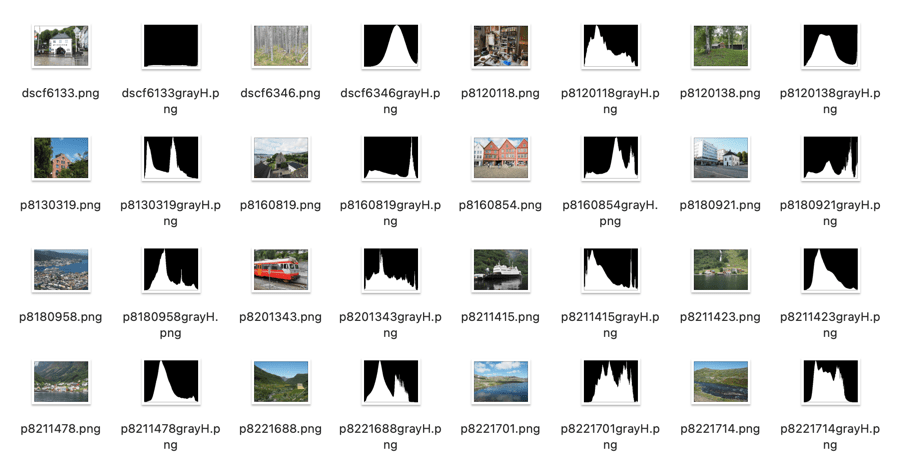
Below is a sample of the output applied to a folder. Now I can easily see what the intensity histogram associated with each image looks like.
Histograms generated using a script.
Yes, some of these seem a bit complicated, but once you have a script it can be easily modified to perform other batch processing tasks.